Have a language expert improve your writing
Run a free plagiarism check in 10 minutes, generate accurate citations for free.
- Knowledge Base
- Frequency Distribution | Tables, Types & Examples

Frequency Distribution | Tables, Types & Examples
Published on June 7, 2022 by Shaun Turney . Revised on June 21, 2023.
A frequency distribution describes the number of observations for each possible value of a variable . Frequency distributions are depicted using graphs and frequency tables.

Table of contents
What is a frequency distribution, how to make a frequency table, how to graph a frequency distribution, other interesting articles, frequently asked questions about frequency distributions.
The frequency of a value is the number of times it occurs in a dataset. A frequency distribution is the pattern of frequencies of a variable. It’s the number of times each possible value of a variable occurs in a dataset.
Types of frequency distributions
There are four types of frequency distributions:
- You can use this type of frequency distribution for categorical variables .
- You can use this type of frequency distribution for quantitative variables .
- You can use this type of frequency distribution for any type of variable when you’re more interested in comparing frequencies than the actual number of observations.
- You can use this type of frequency distribution for ordinal or quantitative variables when you want to understand how often observations fall below certain values .
Receive feedback on language, structure, and formatting
Professional editors proofread and edit your paper by focusing on:
- Academic style
- Vague sentences
- Style consistency
See an example

Frequency distributions are often displayed using frequency tables . A frequency table is an effective way to summarize or organize a dataset. It’s usually composed of two columns:
- The values or class intervals
- Their frequencies
The method for making a frequency table differs between the four types of frequency distributions. You can follow the guides below or use software such as Excel, SPSS, or R to make a frequency table.
How to make an ungrouped frequency table
- For ordinal variables , the values should be ordered from smallest to largest in the table rows.
- For nominal variables , the values can be in any order in the table. You may wish to order them alphabetically or in some other logical order.
- Especially if your dataset is large, it may help to count the frequencies by tallying . Add a third column called “Tally.” As you read the observations, make a tick mark in the appropriate row of the tally column for each observation. Count the tally marks to determine the frequency.

How to make a grouped frequency table
- Calculate the range . Subtract the lowest value in the dataset from the highest.

- Create a table with two columns and as many rows as there are class intervals. Label the first column using the variable name and label the second column “Frequency.” Enter the class intervals in the first column.
- Count the frequencies. The frequencies are the number of observations in each class interval. You can count by tallying if you find it helpful. Enter the frequencies in the second column of the table beside their corresponding class intervals.
| 52, 34, 32, 29, 63, 40, 46, 54, 36, 36, 24, 19, 45, 20, 28, 29, 38, 33, 49, 37 |

Round the class interval width to 10.
The class intervals are 19 ≤ a < 29, 29 ≤ a < 39, 39 ≤ a < 49, 49 ≤ a < 59, and 59 ≤ a < 69.

How to make a relative frequency table
- Create an ungrouped or grouped frequency table .
- Add a third column to the table for the relative frequencies. To calculate the relative frequencies, divide each frequency by the sample size. The sample size is the sum of the frequencies.

How to make a cumulative frequency table
- Create an ungrouped or grouped frequency table for an ordinal or quantitative variable. Cumulative frequencies don’t make sense for nominal variables because the values have no order—one value isn’t more than or less than another value.
- Add a third column to the table for the cumulative frequencies. The cumulative frequency is the number of observations less than or equal to a certain value or class interval. To calculate the relative frequencies, add each frequency to the frequencies in the previous rows.
- Optional: If you want to calculate the cumulative relative frequency , add another column and divide each cumulative frequency by the sample size.

Pie charts, bar charts, and histograms are all ways of graphing frequency distributions. The best choice depends on the type of variable and what you’re trying to communicate.
A pie chart is a graph that shows the relative frequency distribution of a nominal variable .
A pie chart is a circle that’s divided into one slice for each value. The size of the slices shows their relative frequency.
This type of graph can be a good choice when you want to emphasize that one variable is especially frequent or infrequent, or you want to present the overall composition of a variable.
A disadvantage of pie charts is that it’s difficult to see small differences between frequencies. As a result, it’s also not a good option if you want to compare the frequencies of different values.

A bar chart is a graph that shows the frequency or relative frequency distribution of a categorical variable (nominal or ordinal).
The y -axis of the bars shows the frequencies or relative frequencies, and the x -axis shows the values. Each value is represented by a bar, and the length or height of the bar shows the frequency of the value.
A bar chart is a good choice when you want to compare the frequencies of different values. It’s much easier to compare the heights of bars than the angles of pie chart slices.

A histogram is a graph that shows the frequency or relative frequency distribution of a quantitative variable . It looks similar to a bar chart.
The continuous variable is grouped into interval classes , just like a grouped frequency table . The y -axis of the bars shows the frequencies or relative frequencies, and the x -axis shows the interval classes. Each interval class is represented by a bar, and the height of the bar shows the frequency or relative frequency of the interval class.
Although bar charts and histograms are similar, there are important differences:
| Bar chart | Histogram | |
|---|---|---|
| Type of variable | Categorical | Quantitative |
| Value grouping | Ungrouped (values) | Grouped (interval classes) |
| Bar spacing | Can be a space between bars | Never a space between bars |
| Bar order | Can be in any order | Can only be ordered from lowest to highest |
A histogram is an effective visual summary of several important characteristics of a variable. At a glance, you can see a variable’s central tendency and variability , as well as what probability distribution it appears to follow, such as a normal , Poisson , or uniform distribution.

If you want to know more about statistics , methodology , or research bias , make sure to check out some of our other articles with explanations and examples.
- Student’s t table
- Student’s t distribution
- Quartiles & Quantiles
- Measures of central tendency
- Correlation coefficient
Methodology
- Cluster sampling
- Stratified sampling
- Types of interviews
- Cohort study
- Thematic analysis
Research bias
- Implicit bias
- Cognitive bias
- Survivorship bias
- Availability heuristic
- Nonresponse bias
- Regression to the mean
A histogram is an effective way to tell if a frequency distribution appears to have a normal distribution .
Plot a histogram and look at the shape of the bars. If the bars roughly follow a symmetrical bell or hill shape, like the example below, then the distribution is approximately normally distributed.

Categorical variables can be described by a frequency distribution. Quantitative variables can also be described by a frequency distribution, but first they need to be grouped into interval classes .
Probability is the relative frequency over an infinite number of trials.
For example, the probability of a coin landing on heads is .5, meaning that if you flip the coin an infinite number of times, it will land on heads half the time.
Since doing something an infinite number of times is impossible, relative frequency is often used as an estimate of probability. If you flip a coin 1000 times and get 507 heads, the relative frequency, .507, is a good estimate of the probability.
Cite this Scribbr article
If you want to cite this source, you can copy and paste the citation or click the “Cite this Scribbr article” button to automatically add the citation to our free Citation Generator.
Turney, S. (2023, June 21). Frequency Distribution | Tables, Types & Examples. Scribbr. Retrieved September 16, 2024, from https://www.scribbr.com/statistics/frequency-distributions/
Is this article helpful?

Shaun Turney
Other students also liked, variability | calculating range, iqr, variance, standard deviation, types of variables in research & statistics | examples, normal distribution | examples, formulas, & uses, what is your plagiarism score.

An official website of the United States government
The .gov means it’s official. Federal government websites often end in .gov or .mil. Before sharing sensitive information, make sure you’re on a federal government site.
The site is secure. The https:// ensures that you are connecting to the official website and that any information you provide is encrypted and transmitted securely.
- Publications
- Account settings
Preview improvements coming to the PMC website in October 2024. Learn More or Try it out now .
- Advanced Search
- Journal List
- J Pharmacol Pharmacother
- v.2(1); Jan-Mar 2011
Frequency distribution
S manikandan.
Assistant Editor, JPP
INTRODUCTION
The next step after the completion of data collection is to organize the data into a meaningful form so that a trend, if any, emerging out of the data can be seen easily. One of the common methods for organizing data is to construct frequency distribution. Frequency distribution is an organized tabulation/graphical representation of the number of individuals in each category on the scale of measurement.[ 1 ] It allows the researcher to have a glance at the entire data conveniently. It shows whether the observations are high or low and also whether they are concentrated in one area or spread out across the entire scale. Thus, frequency distribution presents a picture of how the individual observations are distributed in the measurement scale.
DISPLAYING FREQUENCY DISTRIBUTIONS
Frequency tables.
A frequency (distribution) table shows the different measurement categories and the number of observations in each category. Before constructing a frequency table, one should have an idea about the range (minimum and maximum values). The range is divided into arbitrary intervals called “class interval.” If the class intervals are too many, then there will be no reduction in the bulkiness of data and minor deviations also become noticeable. On the other hand, if they are very few, then the shape of the distribution itself cannot be determined. Generally, 6–14 intervals are adequate.[ 2 ]
The width of the class can be determined by dividing the range of observations by the number of classes. The following are some guidelines regarding class widths:[ 1 ]
- It is advisable to have equal class widths. Unequal class widths should be used only when large gaps exist in data.
- The class intervals should be mutually exclusive and nonoverlapping.
- Open-ended classes at the lower and upper side (e.g., <10, >100) should be avoided.
The frequency distribution table of the resting pulse rate in healthy individuals is given in Table 1 . It also gives the cumulative and relative frequency that helps to interpret the data more easily.
Frequency distribution of the resting pulse rate in healthy volunteers (N = 63)
| Pulse/min | Frequency | Cumulative frequency | Relative cumulative frequency (%) |
|---|---|---|---|
| 60–64 | 2 | 2 | 3.17 |
| 65–69 | 7 | 9 | 14.29 |
| 70–74 | 11 | 20 | 31.75 |
| 75–79 | 15 | 35 | 55.56 |
| 80–84 | 10 | 45 | 71.43 |
| 85–89 | 9 | 54 | 85.71 |
| 90–94 | 6 | 60 | 95.24 |
| 95–99 | 3 | 63 | 100 |
Frequency distribution graphs
A frequency distribution graph is a diagrammatic illustration of the information in the frequency table.
A histogram is a graphical representation of the variable of interest in the X axis and the number of observations (frequency) in the Y axis. Percentages can be used if the objective is to compare two histograms having different number of subjects. A histogram is used to depict the frequency when data are measured on an interval or a ratio scale. Figure 1 depicts a histogram constructed for the data given in Table 1 .

Histogram of the resting pulse rate in healthy volunteers (N = 63)
A bar diagram and a histogram may look the same but there are three important differences between them:[ 3 , 4 ]
In a histogram, there is no gap between the bars as the variable is continuous. A bar diagram will have space between the bars.
All the bars need not be of equal width in a histogram (depends on the class interval), whereas they are equal in a bar diagram.
The area of each bar corresponds to the frequency in a histogram whereas in a bar diagram, it is the height [ Figure 1 ].
Frequency polygon
A frequency polygon is constructed by connecting all midpoints of the top of the bars in a histogram by a straight line without displaying the bars. A frequency polygon aids in the easy comparison of two frequency distributions. When the total frequency is large and the class intervals are narrow, the frequency polygon becomes a smooth curve known as the frequency curve. A frequency polygon illustrating the data in Table 1 is shown in Figure 2 .

Frequency polygon of the resting pulse rate in healthy volunteers (N = 63)
Box and whisker plot
This graph, first described by Tukey in 1977, can also be used to illustrate the distribution of data. There is a vertical or horizontal rectangle (box), the ends of which correspond to the upper and lower quartiles (75 th and 25 th percentile, respectively). Hence the middle 50% of observations are represented by the box. The length of the box indicates the variability of the data. The line inside the box denotes the median (sometimes marked as a plus sign). The position of the median indicates whether the data are skewed or not. If the median is closer to the upper quartile, then they are negatively skewed and if it is near the lower quartile, then positively skewed.
The lines outside the box on either side are known as whiskers [ Figure 3 ]. These whiskers are 1.5 times the length of the box, i.e., the interquartile range (IQR). The end of whiskers is called the inner fence and any value outside it is an outlier. If the distribution is symmetrical, then the whiskers are of equal length. If the data are sparse on one side, the corresponding side whisker will be short. The outer fence (usually not marked) is at a distance of three times the IQR on either side of the box. The reason behind having the inner and outer fence at 1.5 and 3 times the IQR, respectively, is the fact that 95% of observations fall within 1.5 times the IQR, and it is 99% for 3 times the IQR.[ 5 ]

Schematic diagram of a “box and whisker plot”
CHARACTERISTICS OF FREQUENCY DISTRIBUTION
There are four important characteristics of frequency distribution.[ 6 ] They are as follows:
- Measures of central tendency and location (mean, median, mode)
- Measures of dispersion (range, variance, standard deviation)
- The extent of symmetry/asymmetry (skewness)
- The flatness or peakedness (kurtosis).
These will be dealt with in detail in the next issue.
Source of Support: Nil
Conflict of Interest: None declared
- Skip to secondary menu
- Skip to main content
- Skip to primary sidebar
Statistics By Jim
Making statistics intuitive
Frequency Table: How to Make & Examples
By Jim Frost 2 Comments
What is a Frequency Table?
A frequency table lists a set of values and how often each one appears. Frequency is the number of times a specific data value occurs in your dataset. These tables help you understand which data values are common and which are rare. These tables organize your data and are an effective way to present the results to others. Frequency tables are also known as frequency distributions because they allow you to understand the distribution of values in your dataset.
For example, if 18 students have pet dogs, dog ownership has a frequency of 18. A frequency table of pet ownership will list various types of pets and their frequencies, including dogs.
Frequency distribution tables are a great way to find the mode for datasets.
In this post, learn how to create and interpret frequency tables for different types of data. I’ll also show you the next steps for a more thorough analysis.
How to Make Frequency Distribution Tables for Different Data Types
You can make frequency tables for various types of data, including categorical, ordinal, and continuous. Categorical and ordinal data have natural groupings that you’ll use in the frequency distribution. However, for continuous data, you need to create logical groups for the frequency distribution.
Frequency tables display distributions for one variable, such as type of pet or dining satisfaction. When you need to assess two categorical variables together, use a contingency table instead. Learn more about Contingency Table: Definition, Examples & Interpreting . Statisticians also refer to them as two-way tables .
Let’s go through examples of frequency tables for different data types.
Categorical Data
Categorical data, also known as nominal data , have at least three categories with no natural order. For example, science fiction, drama, and comedy are nominal data .
For categorical data, make a frequency table by counting the number of times each group appears in your dataset.
Imagine you survey a class and ask them to indicate the types of pets they have. Type of pet is a categorical variable. Your raw data might be a list like the following:

From the raw data, count the occurrence of each type of pet and record them in the table. Because the categories don’t have a natural order, you can choose the order to list them in the frequency distribution that makes the most sense for your project. One option is to list the groups from most to least common.
In the example, I list the categories in descending order of occurrence, placing the most popular pets are at the top.

The frequency table indicates that dogs are the most popular type of pet among class members. Fish are rare pets in this class. Ten individuals do not have any pets.
Ordinal Data
Ordinal variables have at least three categories that have a natural order. The groups are ranked, but the differences between them might not be equal. For example, first, second, and third in a race are ordinal data. Learn more about Ordinal Data: Definition, Examples & Analysis .
For ordinal data, make a frequency table by counting the number of times each category occurs in your dataset.
Suppose you survey diners at a restaurant and ask them to rate their dining experience on the following ordinal scale:
- Very satisfied
- Dissatisfied
- Very dissatisfied
Your dataset might look like the following:

From the raw data, count the occurrence of each level of satisfaction and record them in the frequency table. Because the groups have a natural order, list them in the frequency table using that order. In the example, I list the categories in descending order of satisfaction.

The frequency table shows that, on the whole, most diners were very satisfied and satisfied with their experience. However, there were a few diners who were not happy.
Continuous Data
Continuous variables can take on almost any value, and you can divide them meaningfully into smaller increments, such as decimal values. Typically, you’ll measure continuous data on a scale. For example, when you measure height, weight, and temperature, you have continuous data.
Continuous data requires you to create the groups for frequency tables because they can have many distinct values.
Imagine you’re creating a frequency table of heights for 88 participants in a study. Your data will likely have many unique values. Below is a portion of heights in meters from an actual study I conducted involving preteen girls:

If you don’t create groups for continuous data like the example above, your distribution will contain many rows, each with a low count. That’s not going to be very helpful!
To make frequency distribution for continuous data, you’ll need to create groups of values for your continuous data. You can base your groups on ranges of values that make sense for your data when that’s possible. Usually, the spread of values for each group should be equal. In the frequency table, list these groups in ascending order. Groups must be mutually exclusive so that each data point falls into only one group!
Group Frequencies
In a frequency table for continuous data, the group counts indicate the number of times data values fall within each group.
For the height data, I used Excel and its FREQUENCY function to make the frequency table below. You can download the Excel file with the data and table: HeightFrequencyTable .

For the height data, the frequency table indicates that a plurality of values falls near the center of the distribution (1.46 – 1.51m, f = 31). As you move away from the center, the occurrences decrease. The groups with the shortest and tallest heights have the lowest counts, 4 and 6, respectively. You can also see that the overall sample of heights ranges from 1.34 to 1.69m.
Next Steps After Making a Frequency Table
Analysts often create graphs that visually represent a frequency distribution because it gives their report more visual impact. Just like how you alter the frequency tables by the type of data, you’ll need to use various kinds of charts for different data types. Learn more in my post about graphing different types of data .
Making a frequency table is only the first step in understanding the distribution of values in your dataset. To better understand your data’s distribution, consider the following steps:
- Find the cumulative frequency distribution .
- Create a relative frequency distribution .
- Find the central tendency of your data .
- Understand the variability of your data .
- Calculate the descriptive statistics for your sample .
- Identify the probability distribution that your data follow .
Share this:

Reader Interactions

August 17, 2024 at 4:03 am
10 students were interviewed for their result maths course from 100% and the result is 70, 65, 60, 70, 85, 80, 85, 75, 60 and 55. calculate 1. construct frequency table 2. draw bar graph 3. calculate mean, media and mode for it 4. find range 5. calculate mean deviation 6. calculate standard deviation and variance

July 27, 2024 at 8:45 am
very informative.
Comments and Questions Cancel reply
Frequency Distribution Table: Examples, How to Make One
Contents (Click to skip to that section):
What is a Frequency Distribution Table?
- Using Tally Marks
- Including Classes
Types of Frequency Distribution
See also: Frequency Distribution Table in Excel
Watch the video for an example of how to make a frequency distribution table with classes:
Can’t see the video? Click here to watch it on YouTube.
Frequency tells you how often something happened . The frequency of an observation tells you the number of times the observation occurs in the data. For example, in the following list of numbers, the frequency of the number 9 is 5 (because it occurs 5 times):
1, 2, 3, 4, 6, 9, 9, 8, 5, 1, 1, 9, 9, 0, 6, 9.
A frequency distribution is a summary of this type of data [1]. It gives us the number of observations within a specific interval, shown either graphically (usually with a bar chart or a histogram ) or as a f requency distribution table . Frequency in this context indicates the occurrence of a value within a specified interval, while distribution refers to the pattern of the variable’s frequency.
Tables can show either categorical variables (sometimes called qualitative variables ) or quantitative variables (sometimes called numeric variables). You can think of categorical variables as categories (like eye color or brand of dog food) and quantitative variables as numbers.
The following table shows what family planning methods were used by teens in Kweneng, West Botswana. The left column shows the categorical variable (Method) and the right column is the frequency — the number of teens using that particular method.

Frequency distribution tables give you a snapshot of the data to allow you to find patterns. A quick look at the above frequency distribution table tells you the majority of teens don’t use any birth control at all.
Back to Top
How to make a Frequency Distribution Table: Examples
Example 1: Tally marks are often used to make a frequency distribution table. For example, let’s say you survey a number of households and find out how many pets they own. The results are 3, 0, 1, 4, 4, 1, 2, 0, 2, 2, 0, 2, 0, 1, 3, 1, 2, 1, 1, 3. Looking at that string of numbers boggles the eye; a frequency distribution table will make the data easier to understand.

How to Draw a Frequency Distribution Table (Slightly More Complicated Example)
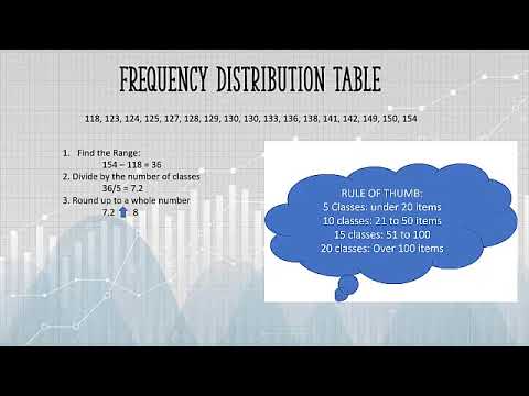
A frequency distribution table is one way you can organize data so that it makes more sense. For example, let’s say you have a list of IQ scores for a gifted classroom in a particular elementary school. The IQ scores are: 118, 123, 124, 125, 127, 128, 129, 130, 130, 133, 136, 138, 141, 142, 149, 150, 154. That list doesn’t tell you much about anything. You could draw a frequency distribution table , which will give a better picture of your data than a simple list.
How to Draw a Frequency Distribution Table: Steps.
Part 1: choosing classes.
Step 1: Figure out how many classes (categories) you need. There are no hard rules about how many classes to pick, but there are a couple of general guidelines:
- Pick between 5 and 20 classes. For the list of IQs above, we picked 5 classes.
- Make sure you have a few items in each category. For example, if you have 20 items, choose 5 classes (4 items per category), not 20 classes (which would give you only 1 item per category).
Note : There is a more mathematical way to choose classes. The formula is log(observations)\ log(2). You would round up the answer to the next integer . For example, log17\log2 = 4.1 will be rounded up to become 5. Another way to do this is with Sturges formula : Number of classes = 1 + 3.322 log N , where N is the number of items in the set.
Part 2: Sorting the Data
Step 2: Subtract the minimum data value from the maximum data value. For example, our IQ list above had a minimum value of 118 and a maximum value of 154, so:
154 – 118 = 36
Step 3: Divide your answer in Step 2 by the number of classes you chose in Step 1.
36 / 5 = 7.2
Step 4: Round the number from Step 3 up to a whole number to get the class width . Rounded up, 7.2 becomes 8 .
Step 5: Write down your lowest value for your first minimum data value:
The lowest value is 118
Step 6: Add the class width from Step 4 to Step 5 to get the next lower class limit:
118 + 8 = 126
Step 7: Repeat Step 6 for the other minimum data values (in other words, keep on adding your class width to your minimum data values) until you have created the number of classes you chose in Step 1. We chose 5 classes, so our 5 minimum data values are:
- 118 126 (118 + 8)
- 134 (126 + 8)
- 142 (134 + 8)
- 150 (142 + 8)
Step 8: Write down the upper class limits. These are the highest values that can be in the category, so in most cases you can subtract 1 from the class width and add that to the minimum data value. For example:
- 118 + (8 – 1) = 125
- 118 – 125
- 126 – 133
- 134 – 141
- 142 – 149 1
- 50 – 157
3. Finishing the Table Up
Step 9: Add a second column for the number of items in each class, and label the columns with appropriate headings:
| IQ | Number |
|---|---|
| 118-125 | |
| 126-133 | |
| 134-141 | |
| 142-149 | |
| 150-157 |
Step 10: Count the number of items in each class, and put the total in the second column. The list of IQ scores are: 118, 123, 124, 125, 127, 128, 129, 130, 130, 133, 136, 138, 141, 142, 149, 150, 154.
| IQ | Number |
|---|---|
| 118-125 | 4 |
| 126-133 | 6 |
| 134-141 | 3 |
| 142-149 | 2 |
| 150-157 | 2 |
That’s How to Draw a Frequency Distribution Table, the easy way!
Tip : If you are working with large numbers (like hundreds or thousands), round Step 4 up to a large whole number that’s easy to make into classes, like 100, 1000, or 10,000. Likewise with very small numbers — you may want to round to 0.1, 0.001 or a similar division.
There are a few variations of frequency distributions:
- Ungrouped frequency distribution : a table that shows the number of data points for each individual value. This is sometimes called just a “frequency distribution.” This is the type shown in example 1 above.
- Grouped frequency distribution : a table that shows the number of data points that fall within a range of values, called a class interval. This type is shown in example 2 above.
- Cumulative frequency distribution : shows the sum of all values up to the current class.
- Relative frequency distribution: shows the proportion of all values that fall within a particular class.
- Relative cumulative frequency distribution: shows the proportion of all values that are less than or equal to a particular value in a frequency distribution.
We can also create a relative frequency marginal distribution, which, shows relative frequencies rather than frequencies for marginal probability distributions [2].
- Blank, B. (2016). Elementary Statistics .
- Section 4.4: Contingency Tables and Association.
Frequency Distribution Table
A frequency distribution table displays the frequency of each data set in an organized way. It helps us to find patterns in the data and also enables us to analyze the data using measures of central tendency and variance. The first step that a mathematician does with the collected data is to organize it in the form of a frequency distribution table. All the calculations and statistical tests and analyses come later.
| 1. | |
| 2. | |
| 3. | |
| 4. | |
| 5. | |
| 6. |
What is a Frequency Distribution Table?
A frequency distribution table is a way to organize data so that it makes the data more meaningful. A frequency distribution table is a chart that summarizes all the data under two columns - variables/categories, and their frequency. It has two or three columns. Usually, the first column lists all the outcomes as individual values or in the form of class intervals, depending upon the size of the data set. The second column includes the tally marks of each outcome. The third column lists the frequency of each outcome. Also, the second column is optional.
Do you know the meaning of "frequency?" Frequency indicates how often something occurs. For example, your heartbeat is 72 heartbeats/min under normal conditions. Frequency corresponds to the number of times a value occurs.
In our day-to-day lives, we come across a lot of information in the form of numerical figures, tables, graphs, etc. This information could be marks scored by students, temperatures of different cities, points scored in matches, etc. The information that is collected is called data . Once the data is collected, we have to represent it in a meaningful manner so that it can be easily understood. The frequency distribution table is one of the ways to organize data.
Here's a frequency distribution table example for you to understand this concept better. Jane is fond of playing games with dice. She throws the dice and notes the observations each time. These are her observations: 4, 6, 1, 2, 2, 5, 6, 6, 5, 4, 2, 3. To know the exact number of times she got each digit (1, 2, 3, 4, 5, 6) as the outcome, she classifies them into categories. An easy way is to draw a frequency distribution table with tally marks.
| Outcomes | Tally Marks | Frequency |
|---|---|---|
| 1 | I | 1 |
| 2 | I I I | 3 |
| 3 | I | 1 |
| 4 | I I | 2 |
| 5 | I I | 2 |
| 6 | I I I | 3 |
The table above is an example of a frequency distribution table. You can observe that all the data that was collected has been organized under three columns. Thus, a frequency distribution table is a chart summarizing the values and their frequencies. In other words, it is a tool to organize data. This makes it easy for us to understand the given set of information.
Thus, the frequency distribution table in statistics helps us to condense data in a simpler form so that it is easy for us to observe its features at a glance.
How to Construct a Frequency Distribution Table?
It is easy to make a frequency distribution table by using the steps given below:
- Step 1: Make a table with two columns - one with the title of the data you are organizing and the other column will be for frequency. [Draw three columns if you want to add tally marks too]
- Step 2: Look at the items written in the data and decide whether you want to draw an ungrouped frequency distribution table or a grouped frequency distribution table. If there are too many different values, then it is usually better to go with the grouped frequency distribution table.
- Step 3: Write the data set values in the first column.
- Step 4: Count how many times each item is repeating itself in the collected data. In other words, find the frequency of each item by counting.
- Step 5: Write the frequency in the second column corresponding to each item.
- Step 6: At last you can also write the total frequency in the last row of the table.
Let's look at an example. Ms. Jennifer is a teacher. She wants to look at the marks obtained by the students of her class in the last exam. She does not have the time to go through each test paper individually to see the marks. Thus, she asks Mr. Thomas to organize the data in a table so that it is easier for her to look at everyone's marks together. Ms. Jennifer suggests using a frequency distribution table to organize the data, so as to get a better picture of the data rather than using a simple list.
Using a frequency distribution table here is a good way to present the data as it will show Ms. Jennifer all the students' marks in one table. But how can a frequency distribution table be created? Mr. Thomas works hard to put together all the data. The following table shows the test scores of 20 students, i.e., for one class.
| Marks obtained in the test | Number of students (Frequency) |
|---|---|
| 9 | 1 |
| 11 | 4 |
| 13 | 1 |
| 18 | 1 |
| 20 | 1 |
| 21 | 2 |
| 22 | 1 |
| 23 | 3 |
| 25 | 1 |
| 26 | 3 |
| 29 | 1 |
| 30 | 1 |
The frequency distribution table drawn above is called an ungrouped frequency distribution table . It is the representation of ungrouped data and is typically used when you have a smaller data set. Imagine how difficult it would be to create a similar table if you have a large number of observations, for example, the marks of students of three classes. The table we will get will be quite lengthy and the data will be confusing.
Hence, in such cases, we form class intervals to tally the frequency for the data that belongs to that specific class interval. To make such a frequency distribution table, first, write the class intervals in one column. Next, tally the numbers in each category based on the number of times it appears. Finally, write the frequency in the final column.
| Marks obtained in the test | Number of students (Frequency) |
|---|---|
| 0 - 5 | 3 |
| 5 - 10 | 11 |
| 10 - 15 | 12 |
| 15 - 20 | 19 |
| 20 - 25 | 7 |
| 25 - 30 | 8 |
A frequency distribution table drawn above is called a grouped frequency distribution table .
What is Frequency Distribution Table in Statistics?
Frequency distribution in statistics is a representation of data displaying the number of observations within a given interval. The representation of a frequency distribution can be graphical or tabular. Now let us look at another way to represent data i.e., graphical representation of data. This is done using a frequency distribution table graph. Such graphs make it easier to understand the collected data.
- Bar graphs represent data using bars of uniform width with equal spacing between them.
- A pie chart shows a whole circle, divided into sectors where each sector is proportional to the information it represents.
- A frequency polygon is drawn by joining the mid-points of the bars in a histogram .
Frequency Distribution Table for Grouped Data
A frequency distribution table for grouped data is known as a grouped frequency distribution table. It is based on the frequencies of class intervals. As it is already discussed above that in this table, all the categories of data are divided into different class intervals of the same width, for example, 0-10, 10-20, 20-30, etc. And then the frequency of that class interval is marked against each interval. Look at an example of the frequency distribution table for grouped data given in the image below.

Cumulative Frequency Distribution Table
Cumulative frequency means the sum of frequencies of the class and all the classes below it. It is calculated by adding the frequency of each class lower than the corresponding class interval or category. An example of a cumulative frequency distribution table is given below:

Cumulative frequency distribution table calculators save a lot of time when tabulating the data. It makes calculations easy and leads to the organization of data in seconds.
Frequency Distribution Table Related Articles
Check these articles related to the concept of a frequency distribution table in math.
- Frequency Distribution
- Frequency Distribution Formula
- Cumulative Frequency
- How To Find Relative Frequency
Frequency Distribution Table Examples
Example 1: A school conducted a blood donation camp. The blood groups of 30 students were recorded as follows.
A, B, O, O, AB, O, A, O, B, A, O, B, A, O, O, A, AB, O, A, A, O, O, AB, B, A, O, B, A, B, O
Represent this data in the form of a frequency distribution table.
Solution: The above data can be represented in a frequency distribution table as follow:
| Blood Group | Number of students |
|---|---|
| A | 9 |
| B | 6 |
| AB | 3 |
| O | 12 |
Example 2: Given below are the weekly pocket expenses (in $) of a group of 25 students selected at random.
37, 41, 39, 34, 41, 26, 46, 31, 48, 32, 44, 39, 35, 39, 37, 49, 27, 37, 33, 38, 49, 45, 44, 37, 36
Construct a grouped frequency distribution table with class intervals of equal widths, starting from 25 - 30, 30 - 35, and so on. Also, find the range of weekly pocket expenses.
Solution: The following table represents the given data:
| Weekly expenses (in $) | Number of students |
|---|---|
| 25-30 | 2 |
| 30-35 | 4 |
| 35-40 | 10 |
| 40-45 | 4 |
| 45-50 | 5 |
In the given data, the smallest value is 26 and the largest value is 49. So, the range of the weekly pocket expenses = 49 - 26 = $23.
Example 3: Silvia and Ashley have a set of number cards with numbers from 1 to 10. They take out a number card and write the number that comes up. They continue doing the same at least 12 times. They get the following values:
5, 8, 9, 2, 3, 7, 3, 4, 5, 9, 3, 1
Construct a frequency table to arrange the data in better form.
| Values | Frequency |
|---|---|
| 1 | 1 |
| 2 | 1 |
| 3 | 3 |
| 4 | 1 |
| 5 | 2 |
| 6 | 0 |
| 7 | 1 |
| 8 | 1 |
| 9 | 2 |
| 10 | 0 |
go to slide go to slide go to slide

Book a Free Trial Class
Practice Questions on Frequency Distribution Table
go to slide go to slide
FAQs on Frequency Distribution Table
What is frequency distribution table.
A frequency distribution table is a tabular representation of the frequencies of the categories given. It represents the data in an organized manner that is useful for the graphical representation of data or to calculate mean, median, and mode , variance , etc. It has generally two columns, one is of the categories of data set, and the other one is of the frequency of each category. Sometimes, a tally marks column is also added before frequency that helps to count the frequency.
What is the Use of a Frequency Distribution Table?
A frequency distribution table is useful to perform calculations on the given data. It involves calculations involving measures of central tendency , variance, statistical tests, and analysis. Apart from that, a frequency distribution table is useful to represent the data in a neat manner that is easy to understand.
How to Make an Ungrouped Frequency Distribution Table?
To make an ungrouped frequency distribution table, follow the steps given below:
- Identify all the categories that are given in the data.
- Draw a table with two columns - one is of categories and another is of their respective frequencies. Draw three columns if you want to add tally marks too.
- Write each category in a separate row in column 1.
- Count the number of times they are occurring or repeating themselves in the collected data.
- Write those frequencies for each category in column 2.
What is Grouped Frequency Distribution Table?
A grouped frequency distribution table is a table that represents categories in the form of class intervals. It is mainly used with large data sets.
What is cf in Frequency Distribution Table?
In a frequency distribution table, cf means cumulative frequency. Cf represents the collective or total frequency of a category and all the categories lower or greater than that.
How to Interpret Frequency Distribution Table?
The following points must be kept in mind while interpreting a frequency distribution table:
- The first column is usually for the categories of the data set and the second or third column is usually for the frequency of each category.
- The number written on the right of each category is its frequency. It lies in the same row.
- There are no other category lies except the ones written in the first column of the table.
How to Draw Frequency Distribution Table?
There are mainly two or three columns in a frequency distribution table - column 1 for categories, column 2 for tally marks, and column 3 for frequency. So, to draw a frequency distribution table, we have to write data in this order only. First, we identify all the categories or class intervals, then we write them in separate rows in column 1. After that, we focus on each category one by one and count their frequencies. We write their respective frequency in the third column. This is how we can draw a frequency distribution table.
How to Get Class Boundary in Frequency Distribution Table?
A class boundary is a number that separates the class intervals without leaving any gaps. For example, if the two subsequent class intervals are given as 20-29 and 30-39. The class boundary is calculated as (upper limit of the first class interval + lower limit of the second class interval)/2. So, here class boundary = (29+30)/2, which is equal to 29.5.
What are the Types of Frequency Distribution Table?
There are mainly three types of frequency distribution table, which are given below:
- Ungrouped frequency distribution table
- Grouped frequency distribution table
- Cumulative frequency distribution table
- Bipolar Disorder
- Therapy Center
- When To See a Therapist
- Types of Therapy
- Best Online Therapy
- Best Couples Therapy
- Managing Stress
- Sleep and Dreaming
- Understanding Emotions
- Self-Improvement
- Healthy Relationships
- Student Resources
- Personality Types
- Sweepstakes
- Guided Meditations
- Verywell Mind Insights
- 2024 Verywell Mind 25
- Mental Health in the Classroom
- Editorial Process
- Meet Our Review Board
- Crisis Support
What Is a Frequency Distribution In Psychology?
Jeffrey Coolidge / The Image Bank / Getty Images
Understanding how often things happen can be important when researchers are investigating a problem or phenomenon. To learn more, they may use a type of descriptive statistic known as a frequency distribution. A frequency distribution, also known as a frequency table, summarizes how often different scores occur within a sample of scores.
Frequency distributions are presented as a table with each category on the left and the number of each occurrence on the bottom. This allows researchers to conveniently get a quick look at what the overall data shows.
At a Glance
Frequency distributions are often used to help researchers make sense of large amounts of complex data. Rather than focusing on individual data point, researchers may track how often each one occurs. This can provide a quick visual way to understand the data and make it easier to spot patterns.
What Is a Frequency Distribution?
- A frequency can be defined as how often something happens. For example, the number of dogs that people own in a neighborhood is a frequency.
- A distribution refers to the pattern of these frequencies.
- A frequency distribution looks at how frequently certain things happen within a sample of values. In our example above, you might do a survey of your neighborhood to see how many dogs each household owns.
A frequency distribution is commonly used to categorize information so that it can be interpreted in a visual way.
Why Frequency Distributions Are Helpful
Frequency distributions are a helpful way of presenting complex data. In psychology research , a frequency distribution might be utilized to take a closer look at the meaning behind numbers. For example, imagine that a psychologist was interested in looking at how test anxiety impacted grades.
Rather than simply looking at a huge number of test scores, the researcher might compile the data into a frequency distribution which can then be easily converted into a bar graph. By doing this, the researcher can then quickly look at essential things such as the range of scores and which scores occurred the most and least frequently.
Example of a Frequency Distribution
Let’s say you obtain the following set of scores from your sample:
1, 0, 1, 4, 1, 2, 0, 3, 0, 2, 1, 1, 2, 0, 1, 1, 3
The first step in turning this into a frequency distribution is to create a table. Label one column the items you are counting, in this case, the number of dogs in households in your neighborhood.
Next, create a column where you can tally the responses. Place a line for each instance the number occurs.
Finally, total your tallies and add the final number to a third column.
|
|
|
0 | |||| | 4 |
1 | ||||| || | 7 |
2 | ||| | 3 |
3 | || | 2 |
4 or more | | | 1 |
Using a frequency distribution, you can look for patterns in the data. Looking at the table above you can quickly see that out of the 17 households surveyed, seven families had one dog while four families did not have a dog.
Another Example of a Frequency Distribution
For example, let’s suppose that you are collecting data on how many hours of sleep college students get each night. After conducting a survey of 30 of your classmates, you are left with the following set of scores:
7, 5, 8, 9, 4, 10, 7, 9, 9, 6, 5, 11, 6, 5, 9, 9, 8, 6, 9, 7, 9, 8, 4, 7, 8, 7, 6, 10, 4, 8
In order to make sense of this information, you need to find a way to organize the data. In our example above, the number of hours each week serves as the categories, and the occurrences of each number are then tallied.
The above information could be presented in a table:
|
|
|
4 | ||| | 3 |
5 | ||| | 3 |
6 | |||| | 4 |
7 | ||||| | 5 |
8 | ||||| | 5 |
9 | ||||| | | 7 |
10 | || | 2 |
11 | | | 1 |
Looking at the table, you can quickly see that seven people reported sleeping for 9 hours while only three people reported sleeping for 4 hours.
How Are Frequency Distributions Displayed?
Using the information from a frequency distribution, researchers can then calculate the mean , median , mode, range, and standard deviation. Frequency distributions are often displayed in a table format, but they can also be presented graphically using a histogram.
What This Means For You
If you need to display a large amount of data in a way that is quick and easy to interpret, frequency distributions can be a great choice. This can be important when researchers are trying to spot patterns in a population that might point to a specific problem or solution. Knowing what these tables mean can also help you interpret such research when you come across it in your own studies.
American Psychological Association. Frequency distribution .
Manikandan S. Frequency distribution . J Pharmacol Pharmacother . 2011;2(1):54-56. doi:10.4103/0976-500X.77120
Cooksey RW. Descriptive statistics for summarising data . Illustrating Statistical Procedures: Finding Meaning in Quantitative Data . 2020;61-139. doi:10.1007/978-981-15-2537-7_5
Blair-Broeker CT, Ernst RM, Myers DG. Thinking About Psychology: The Science of Mind and Behavior . New York: Macmillan; 2008.
Cohen BH. Explaining Psychological Statistics . 4th ed. New York: Wiley; 2013.
By Kendra Cherry, MSEd Kendra Cherry, MS, is a psychosocial rehabilitation specialist, psychology educator, and author of the "Everything Psychology Book."

Want to create or adapt books like this? Learn more about how Pressbooks supports open publishing practices.
Goodness of Fit and Related Chi-Square Tests
13 Frequency Distributions
13.1 analyzing distributions of data.
Throughout this text, we will focus on using frequency analysis and descriptive statistics. These simple but powerful analyses enable you to examine your data and identify patterns including the shapes and distributions of data, missing values, and outliers. Frequencies and distributions are important concepts in the quantitative analysis of data that underlie the overall statistical approach covered in this book. In fact, this approach is often referred to as “frequentist statistics” because it relies on frequencies to make inferences about the data. An alternative approach is called the Bayesian statistical analysis which relies on probabilities. While we won’t go into detail about the differences between frequentist and Bayesian statistical approaches, it is important to recognize that frequencies play a key role in the approach that we are demonstrating here but that a frequentist approach is not the only way to analyze your data.
A frequency is simply the number of times something happens. It could be, for example, the number of people with brown hair, the number of children in a family, the number of deaths in a hospital. It could also be the number of times an electrical signal with a given level of energy-intensity is recorded.
A distribution shows the relative frequencies of each possible value or category for a variable. Distributions are used to describe the organization or shape of a set of scores or values for a particular variable. If you studied statistics previously you are most likely familiar with the normal distribution or bell curve. What you may not realize is that distributions other than the normal distribution are also used in statistic analyses and that datasets can take the shape of these other distributions. For example, datasets that include only discrete scores ranging from 1 to 5 would not be expected to fit a normal distribution curve but would rather be compared to a categorical distribution curve – like the chi-square distribution or the Poisson distribution.
Distributions can be obtained by counting the number of events that occur or how many participants in a sample have a specific score on a questionnaire or measure (i.e., counting frequencies). For example, you might look at the number of patients presenting to the Emergency Department for different reasons: cardiovascular concerns, accidents, infections, reported symptoms. You might also consider responses to an anxiety questionnaire scored on a Likert scale (using discrete scaled scores) ranging from 1 to 5. You may consider reviewing the number of respondents in your sample had each possible score (i.e. 1, 2, 3, 4, or 5) – in other words, how frequent each score appeared within the total set of scores.
The following is an example of a table showing a frequency distribution for a set of responses to a categorical variable ranging from 1 to 5, and a graphical representation of the frequency of responses in each category. The Category Label is presented on the x-axis, and the number of responses—frequencies for each response are presented on the y-axis.
Table 13.1 Frequency Distribution For Categorical Responses
The PROC FREQ Procedure
| 22 | 14.77 | 22 | 14.77 | |
| 32 | 21.48 | 54 | 36.24 | |
| 42 | 28.19 | 96 | 64.43 | |
| 35 | 23.49 | 131 | 87.92 | |
| 18 | 12.08 | 149 | 100.00 |
SAS Code to produce the Frequency Distribution and Corresponding Figure
Figure 13.1 Frequency Distribution For a Categorical Response Variable
Frequency distributions are useful in describing variables, helping to identify errors (impossible values) and outliers, assessing how well a continuous variable fits the normal distribution, or to test hypotheses using specific statistical tests such as using a chi-square test to evaluate categorical variables.
Frequency & Distribution of a Count Variable
Count variables refer to those that simply tally the number of items or events that occur. For example, you might want to count the number of adverse events that occur when people take a medication, the number of times nurses wash their hands during their shift or the number of babies born in each month of the year. In health research, there are many items or events that can be counted!
Note that for a count variable, the values are arithmetically meaningful and represent the number of events or items for a specific variable– the count variable is quite literally storing the count of items of interest. Therefore, values differ by a magnitude and are meaningful. For example, 4 adverse events are twice as many as 2 adverse events.
Count variables are different than categorical variables.
Categorical variables are used when the researcher wishes to use numbers to represent different kinds of items or events. In the categorical variable the numbers are arbitrary. For example, hair colour could be coded as 1 = blonde, 2 = brown, 3 = gray, 4 = red, and 5 = other but it could also be coded as 11 = blonde, 22 = brown, 33 = gray, 44 = red, and 55 = other. The numbers representing a category label are not mathematically meaningful and do not represent the number of people with a specific hair colour. Of course, you can analyze the frequency of people with each response which we will cover later when we talk about categorical variables in more detail.
Working example to process a “count” variable
Let’s say we would like to take a sample of 50 families from a population of 1000 households in a small town and record the number of children in each household. Here we will create two variables, the first we will call “ NKIDS ” and the second we will call “ HOUSEHOLDS ”. The variable NKIDS is the categorical variable for the number of children in each household that we sampled, while the variable HOUSEHOLDS represents the number of response houses that report having a given number of children.
The Scenario
We arrive at the small town and knock on the front door of the first house. Below is the dialogue between the researchers and the respondents.
“Good day, we are Biostatisticians and we are conducting a study of the number of children in your family.”
“Oh we don’t have any children.”
“Okay, thank-you.”
We note that for Household #1 there are 0 children. We then knock on the front door of the second house.
“We have 7 children. Would you like some?”
“No thank-you, but have a nice day.”
We note that for Household #2 there are 7 children. We then knock on the front door of the third house, and continue our process for each of 50 houses in the town.
In this example, the categorical variable is NKIDS and is considered the independent variable, while the continuous-discrete variable is HOUSEHOLDS and is considered the dependent variable – aka the measure of interest.
Since there can only be whole numbers for the variable NKIDS (i.e., you can’t actually have 1.2 children), the variable NKIDS is a discrete categorical variable, and likewise, because we are counting families on a whole number line (i.e. not partial families) then the variable NFAMILIES is a discrete random variable.
The frequency distribution recording sheet for this example is shown below. Notice that as a rule, we want to keep our variable labels at or near 8 characters so that HOUSEHOLDS is shortened to HSEHLD.
Table 13.2 Tally Sheet to produce the Frequency Distribution for Number of Children in Each Household Sampled
| Number of Children | Tally of Households | Frequency (f) | Relative frequency (f/n) |
| 0 | ||||| |||| | 9 | 9/50 = 0.18 |
| 1 | ||||| || | 7 | 7/50 = 0.14 |
| 2 | ||||| ||||| || | 12 | 12/50 = 0.24 |
| 3 | ||||| |||| | 9 | 9/50 = 0.18 |
| 4 | ||||| | 5 | 5/50 = 0.10 |
| 5 | ||||| | | 6 | 6/50 = 0.12 |
| 6 | —- | 0 | 0/50 = 0 |
| 7 | || | 2 | 2/50 = 0.04 |
| N=50 | Proportion = 1.00 |
Counting events such as the number of children in a family, the number of needles found on the ground near a safe injection site, or the number of patients readmitted to the hospital after discharge, typically follow the whole number line. Frequency tables are often used to show how many times an event has occurred.
In our example, we can say that the variable HOUSEHOLDS is a discrete random variable because in a given sample of 50 families the variable can take on (contain) any value between 0 and 50 (the total sample) on the whole number line.
Table 13.1 shows how we can determine the frequency and relative frequency (percentage out of 100) for the number of children in each of the families in our sample. Of the 50 families in our sample, nine families did not have children, 7 families had 1 child, 12 families had 2 children, 9 families had 3 children, 5 families had 4 children, 6 families had 5 children, no families had 6 children, and 2 families had 7 children. Notice here that the variable of interest is the number of families reporting each of the possible number of children.
Relative frequency refers to the proportion of the entire sample that had a particular value. In this example, the relative frequency tells us what percentage of the sample had a specific number of children. To calculate the relative frequency, simply divide each frequency by the total number of families and then multiply the result by 100 to calculate the percentage value. For example, from the data in Table 4.1 we see that in this sample, 24% of the families had 2 children while only 4% had 7 children.
Creating the SAS Program to compute a frequency distribution for a discrete random variable
Below are the SAS commands to produce the frequency distribution table of the data recorded for the number of children in our sample of 50 families.
SAS Code to produce a Frequency Distribution Table For Number of Children in Each Household sampled
In this SAS program, we are using the PROC FREQ statistical processing command with the keyword TABLES to produce a frequency distribution for the data recorded for our sample of 50 households. Notice in the PROC FREQ command sequence we included the statement WEIGHT HSEHLD. In this example, the independent or categorical variable is NKIDS and the dependent discrete random variable is HSEHLD. The WEIGHT command enables us to enter the summary data for the dependent variable HSEHLD as the count related to the categorical variable NKIDS.
Notice the table indicates that 9 households reported no children, while no households reported having 6 children. The table also indicates that most households reported having 2 children.
TABLE 13.3 Frequency distribution for number of children in each household
The FREQ Procedure
| NKIDS | Frequency | Percent | Cumulative Frequency | Cumulative Percent |
| 0 | 9 | 18.00 | 9 | 18.00 |
| 1 | 7 | 14.00 | 16 | 32.00 |
| 2 | 12 | 24.00 | 28 | 56.00 |
| 3 | 9 | 18.00 | 37 | 74.00 |
| 4 | 5 | 10.00 | 42 | 84.00 |
| 5 | 6 | 12.00 | 48 | 96.00 |
| 7 | 2 | 4.00 | 50 | 100.00 |
The following is a SAS program to compute elements of PROC FREQ for frequency distributions. The data are fictitious and are used here to enable you to work through the various options and features of the PROC FREQ command with relevant options.
As you work through the SAS program take note of the specific features that are identified, therein. The scenario is based on a public health study in which a group of researchers intended to determine the number of discarded needles left on the ground within a 100-metre radius of safe injection sites. We begin the program first by reading the data set and then using the essential SAS statistical processing commands with relevant options for PROC FREQ.
The program begins by labeling the working SAS program as DATA FREQ13_4; – which simply creates a label for the SAS program in the present SAS work session;
The second line is the listing of variables to be read within the sample data set. The SAS command begins with the SAS keyword INPUT which is followed by the names of each variable. Notice that the variable names are kept to eight characters and each variable name begins with an alphabetic character rather than a number or a special character. In this example the variables SITE, NDLCNT and INCREG are used to indicate that we have a variable to list the various sites from which the data were collected (SITE), the number of needles found on the ground within a 100-metre radius of the exit door of the safe injection site (NDLCNT), and the estimated average household income reported in thousands of dollars for the region in which the injection site is located (INCREG).
We also use simple IF-THEN logic commands to create summary groups for both the variable NDLCNT – number of needles recorded at each site, as well as to group the average household income – INCGRP.
SAS Code to Demonstrate Features of PROC FREQ
F REQUENCY DISTRIBUTION FOR THE NUMBER NEEDLES FOUND ACROSS ALL SITES
| Frequency of Needle Count | ||||
| Needle Count | Frequency | Percent | Cumulative Frequency | Cumulative Percent |
| 0 | 3 | 15.00 | 3 | 15.00 |
| 3 | 2 | 10.00 | 5 | 25.00 |
| 4 | 5 | 25.00 | 10 | 50.00 |
| 5 | 1 | 5.00 | 11 | 55.00 |
| 6 | 2 | 10.00 | 13 | 65.00 |
| 7 | 2 | 10.00 | 15 | 75.00 |
| 8 | 1 | 5.00 | 16 | 80.00 |
| 10 | 4 | 20.00 | 20 | 100.00 |
The SAS commands to sort the data and run the PROC FREQ using the * between variables helps to summarize the data into 2-way frequency distribution tables. In this way, we can see at a glance, a summary of the dataset.
In the sequence of SAS processing commands, we first sort the data using PROC SORT, followed by the SAS commands PROC FREQ with the keyword TABLES and then the two variables that we wish to include in the 2-way table – NDLGRP * INCGRP.
Code Snippet for SAS Code to Demonstrate PROC SORT code added to PROC FREQ
PROC SORT; BY INCGRP; PROC FREQ; TABLES NDLGRP*INCGRP; TITLE1 ‘FREQ DIST FOR GROUP NEEDLES BY INCOME GROUP’; RUN;
The result of this sequence of commands enables us to produce the 2-way SAS table of the groups of needles found arranged by income groups. The problem with this table is that the delivery of information is not optimized for the reader if the reader does not know what an income group of 5, or an NDLGRP of 3 refers.
Using the PROC FORMAT command enables us to explain the categories within each variable. The code to explain the levels of each category uses the following two-step approach.
1.) At the start of the program add the PROC FORMAT statement and the VALUE for each categorical variable.
In our example, we have two categorical variables: INCGRP and NDLGRP. The variable INCGRP has 5 levels, while the variable NDLGRP has three groups.
| PROC FORMAT; VALUE INC 1=’LESS THAN $25K’ 2=’$25K TO $50K’ 3=’$50K TO $75K’ 4=’$75K TO $100K’ 5=’MORE THAN $100K’; VALUE NDL 1 = ‘<=5 NDLS’ 2= ‘6 TO 10 NDLS’ 3= ‘>10 NDLS’; DATA TAB4_3; INPUT SITE NDLCNT INCOME; |
Later in the program, after we call a SAS procedure, like in this case we call PROC FREQ, we then call the FORMAT function and assign the predefined format to each variable used by the SAS procedure.
Notice we first call the variable – in this example the variable of interest is NDLGRP and this is followed by the PROC FORMAT VALUE name NDL. Notice also that when we include the VALUE name we follow it with a period(.). This command will place the full text for the variable category in the frequency distribution.
|
|
The results of this analysis demonstrate that the highest number of needles found near the areas of safe injection sites tended to be higher among low-income neighborhoods than the number of needles found near the safe injection sites located in more affluent areas.
Figure 13.5 Features of Proc Freq: Adding Proc Format to the Frequency Procedure for a block chart
In the following output the SAS syntax is shown here.
At the top of the program add:
13.2 Distribution for a categorical variable
As previously discussed, categorical variables involve grouping items, persons, or attributes, whereby the assignment of numbers to each group is arbitrary. For example, you might be interested in looking at the employment status of nursing home workers. The variable: employment status would be a categorical or grouping variable and might contain the following categories: full-time, part-time, casual, and temporary . You could assign any number you wish to represent the group label because the number is merely a label when applied to represent the category and doesn’t hold any mathematical significance – the number simply enables you to group persons based on that variable (in this case, employment status).
It is important to remember that with categorical data our interest is not to compute measures of centrality or variance like means and standard deviations, and therefore we won’t compare the distribution of items of persons to a normal distribution (i.e., the bell curve). Rather, the data that is held in the categories are counts and so our evaluation approach is to use statistical methods based on frequencies and ranks.
In the following steps, we calculate frequencies, relative frequencies, proportions, and percentages for categorical variables. Consider this simple data set.
| Participant ID | Employment Status | Code |
| 01 | Casual | 3 |
| 02 | Full-time | 1 |
| 03 | Part-time | 2 |
| 04 | Casual | 3 |
| 05 | Casual | 3 |
| 06 | Full-time | 1 |
| 07 | Part-time | 1 |
| 08 | Part-time | 2 |
| 09 | Casual | 3 |
| 10 | Casual | 3 |
We add up how many participants are in each employment status group and transfer the information to our chart:
| 1 | ||| | 3 | 3/10= 0.30 | 30% |
| 2 | || | 2 | 2/10 = 0.20 | 50% |
| 3 | |||| | 5 | 5/10 = 0.50 | 100% |
Better yet, here we will use SAS to produce a frequency distribution table.
SAS code to produce a frequency distribution for employment status
This program produces the basic frequency distribution table for a set of categorical data and since we included the PROC FORMAT commands we can explain the data output clearly.
Features of Proc Freq: Distribution for a Categorical Variable
FREQUENCY DISTRIBUTION OF EMPLOYMENT STATUS
The FREQ Procedure for Employment Status
| 3 | 30.00 | 3 | 30.00 | |
| 2 | 20.00 | 5 | 50.00 | |
| 5 | 50.00 | 10 | 100.00 |
Distribution for a continuous variable
Now let’s talk about analyzing data for continuous variables.
Suppose we recorded the heights (in inches) of 200 students. In this example, height is a continuous variable since the possible values include decimals (not just whole numbers), there are equal intervals between each line on a tape measure, and there is a meaningful 0.
While we can examine frequencies and create a histogram for a continuous variable, it is likely that we will have many different values in our dataset because each student will have a slightly different height. For example, Tom might be 61.5 inches tall while Cara is 61.6 inches tall. As a result, few students will record the exact same height. It may be, therefore, more meaningful to group these data and create categories. In other words, you can transform a continuous variable into a categorical variable simply by grouping the data with the IF-THEN logic statements.
In the following example, we will use the grouping approach so that we can create a more comprehensive frequency distribution.
Let’s start with a dataset that includes two variables for our sample of 200 students (ID and HEIGHT). For each participant, we assign an ID and then record the height in inches for each of our participants. (note: despite that in Canada we use the metric scale for most of our measurements, we continue to refer to our heights in inches and feet – old habits die hard!)
Here we can use SAS to produce the frequency distribution table based on our grouping strategy for the data. We start by naming the working file and then include the appropriate SYNTAX to describe the variables and add the simple logic statements.
Raw Dataset 13.1 Two-hundred Height Measurements (inches)
Below is the SAS code required for the frequency analysis for the dataset above:
PROC FORMAT; VALUE HT 1=’LESS THAN 66.0′ 2=’66.1 TO 68.0′ 3=’68.1 TO 70.0′ 4=’70.1 TO 72.0′ 5=’MORE THAN 72.0′; DATA HEIGHTS; LABEL ID = ‘PARTICIPANT ID’ HEIGHT = ‘PARTICIPANT HEIGHT’ HTGRP=’HEIGHT GROUP’; INPUT ID HEIGHT @@;
Notice some specific features of the INPUT statement above. Here we list two variables: ID and HEIGHT, followed by two @ symbols at the end of the list of variables. When two @ symbols are presented together SAS does not skip to a new line after reading the list of variables (in this case ID and HEIGHT), but rather reads across the page. This format enables us to read the data as a constant stream across the page for as many rows as is required to present the entire dataset. The computer reads the data in the order of the variables listed. That is, the computer reads through the dataset assigning the first value as the ID and the second value as the HEIGHT until all data are read.
Below is the paragraph of simple logic statements that follow the INPUT format statement. With these simple IF-THEN logic statements we organize the large unwieldy data set into six manageable groups.
IF HEIGHT <=66.0 THEN HTGRP=1; IF HEIGHT >66.0 AND HEIGHT <=68.0 THEN HTGRP=2; IF HEIGHT >68.0 AND HEIGHT <=70.0 THEN HTGRP=3; IF HEIGHT >70.0 AND HEIGHT <=72.0 THEN HTGRP=4; IF HEIGHT >72.0 THEN HTGRP=5; DATALINES; 001 58.5 002 58.8 003 60.1 004 61.3 005 61.75 006 61.96 . . .
199 79.40 200 79.47 ; PROC FREQ; TABLES HEIGHT; RUN; PROC FREQ; TABLES HTGRP; FORMAT HTGRP HT. ; RUN;
As you see in the partial output presented in Figure 13.4 below, when we run the SAS command: PROC FREQ; TABLES HEIGHT; RUN; most of the values occur only once because height is a continuous variable which allows greater variation than categorical or count type variables. When reading this output, make sure that you screen for outliers by looking at the high and low values for the variable. SAS will also indicate the number of missing values which is also important when you are cleaning and screening your data.
Table 13.4 The output from PROC FREQ Applied to Continuous Data –Participant Height.
| 1 | 0.50 | 1 | 0.50 | |
| 1 | 0.50 | 2 | 1.00 | |
| 1 | 0.50 | 3 | 1.50 | |
| 1 | 0.50 | 198 | 99.00 | |
| 1 | 0.50 | 199 | 99.50 | |
| 1 | 0.50 | 200 | 100.00 |
13.3 Creating a Histogram in SAS
Producing graphs in SAS enables us to examine the distribution of the data visually rather than in a table. The SAS code shown here includes the option to produce a histogram. A histogram is more than a vertical bar chart. Histograms use rectangles to illustrate the frequency and interval, whereby the height of the rectangle is relative to the frequency (y axis) and the width of the rectangle is relative to the interval (x axis).
The SAS code used here provides the analysis for our sample of 200 measures of height within a cohort of children. In order to establish the appropriate number of intervals in our sample we calculate the range of our set of scores. The range refers to the spread of scores between the lowest estimate from our sample, and the highest estimate from our sample. We can estimate the range apriori by running the PROC UNIVARIATE command. When we include the command MIDPOINTS= we can customize the output. Here we include the command HISTOGRAM /MIDPOINTS = 55 TO 85 BY 0.5, to produce the expected RANGE of highest and lowest values and then plot the midpoints for all categories within the range.
PROC UNIVARIATE; VAR HEIGHT; HISTOGRAM / MIDPOINTS=55 TO 85 BY 0.5 NORMAL; RUN;
Notice in Figure 13.6 that the x-axis is a continuous variable. An overlay of the shape of the distribution is represented by the blue BELL-SHAPED normal curve.
Figure 13.6 Histogram for Heights of Students in Sample of 200 Participants
Use the following SAS Code to group the data into categories and add a representation of the shape of the distribution (CTEXT = BLUE) when plotting the histogram.
proc univariate; var HEIGHT; histogram HEIGHT / normal midpoints = 55 60 65 70 75 80 85 90 CTEXT = BLUE;
Of you can use: proc sgplot; histogram HEIGHT; density HEIGHT;
Figure 13.7 Histogram for Heights of Students N= 200 Grouped Data
Dividing a continuous variable into categories
In the example shown above, it is easy to see how helpful it is to arrange these continuous data into categories that represent a range of values rather than individual values on a continuum.
In our height example, we can optimize these data by creating height categories rather than exact heights because there is so much variance in exact heights. However, in this process of arbitrarily categorizing our response variable by grouping the data together we recognize that there will be a loss of information. When grouping data we are essentially saying that the responses are exactly the same even though differences are observed. For example, when you group a student who is 61.5 inches tall with a student who is 64 inches tall, the difference between the two individuals will be ignored within the category. There is absolutely nothing wrong with using categories that represent a range of continuous values but if you are planning to collect your own data, it is usually best to collect continuous data from the source and group the data later. Generally speaking, you can always convert data from continuous data to categories but without the original estimates, you cannot go the other way!
Once you deem it helpful to transform a continuous variable into categories, next you need to decide how to chop up your data. Ideally each you should have an equal range of values in each group. In our example, which you can see the would-be participants are quite tall, we decided to transform the continuous height data into categories that are each 2 inches wide. Group 1 includes students with a height of less than 66 inches, Group 2 starts at 66.1 and tops out at 68 inches, Group 3 starts at 68.1 and tops out at 70 inches … and so on.
Alternatively, we could have decided to group students in intervals of 5 inches or even 1 inch. As the researcher, you decide how to group the data based on what will make meaningful groupings. This might be based on past literature, clinical reference values, logic, or a combination of these factors. Once we create our categories we can sort students into each group based on their height. Then we can count how many students fall into each group and create a frequency distribution table (Table 13.5) and a histogram. Notice that the shape (distribution) of this histogram is the one we created using the continuous version of the height variable (Figure 13.6). This is because in the first histogram exact values are included and the data is divided into quintiles based on the mean. On the other hand, in the second histogram students are grouped together in 2-inch height intervals – depending on the cut-off values that we chose the distribution would be different.
Using the grouping routines with simple logic statements helps to simplify the organization of the data. The output for the grouped data is invoked with the SAS command: PROC FREQ; TABLES HTGRP; FORMAT HTGRP HT. ; RUN;
Table 13.5 Grouping PROC FREQ output for –Participant Height.
| HTGRP | Frequency | Percent | Cumulative Frequency | Cumulative Percent |
| LESS THAN 66.0 | 40 | 20.00 | 40 | 20.00 |
| 66.1 TO 68.0 | 43 | 21.50 | 83 | 41.50 |
| 68.1 TO 70.0 | 30 | 15.00 | 113 | 56.50 |
| 70.1 TO 72.0 | 48 | 24.00 | 161 | 80.50 |
| MORE THAN 72.0 | 39 | 19.50 | 200 | 100.00 |
Figure 13.7 Histogram for Heights of Students using Height Group (N=200)
In addition to the histogram, SAS also includes a number of tables in the output with the PROC UNIVARIATE command. The data in these tables provide important information about our variable (height, in this example). As you can see in Table 13.8 the moments’ table provides descriptive statistics about our variable including the mean, standard deviation, and standard error, as well as the overall variance. Skewness and kurtosis are also provided which provide valuable information about how well the variable fits the normal distribution. Keep your critical thinking hat on when looking at these data because some of this information is not relevant for categorical variables. For example, you cannot have an average for a categorical variable and the normal distribution doesn’t make sense.
Table 13.8 Descriptive Statistics for the Dataset of Heights
| N | 200 | Sum Weights | 200 |
|---|---|---|---|
| Mean | 69.1297 | Sum Observations | 13825.94 |
| Std Deviation | 3.66230697 | Variance | 13.4124924 |
| Skewness | 0.00184013 | Kurtosis | 0.45301492 |
| Uncorrected SS | 958452.17 | Corrected SS | 2669.08598 |
| Coeff Variation | 5.29773306 | Std Error Mean | 0.25896421 |
The next table presents the Basic Statistical Measures (Figure 13.9). In addition to the mean, standard deviation, and variance, this table also provides the median, mode, range, and interquartile range for the variable.
Table 13.9 Basic Statistical Measures Table
| Median | 69.18500 | Variance | 13.41249 |
|---|---|---|---|
| Mode | 67.72000 | Range | 20.97000 |
| Interquartile Range | 4.54000 | ||
| Location | Variability | ||
| Mean | 69.12970 | Std Deviation | 3.66231 |
Finally, Table 13.10 is the Extreme Observations Table which identifies the highest and lowest values of the variable. Here the data do not differ from what we would expect but when datasets contain outliers, this table is one way to identify the outlier data points easily. Notice that the table provides the case number along with the data point value, making it easy to revisit the original dataset and verify original values or consider adjustments to extreme values if needed.
Figure 13.10 Extreme Observations Table
| Lowest | Highest | ||
| Value | Observation | Value | Observation |
| 58.50 | 1 | 76.34 | 1 |
| 58.80 | 2 | 76.45 | 2 |
| 60.10 | 3 | 78.59 | 3 |
| 61.30 | 4 | 79.25 | 4 |
| 61.75 | 5 | 79.40 | 5 |
Below is a SAS program to produce a graphical presentation of the data while also creating an organized frequency distribution table.
OPTIONS PAGESIZE=55 LINESIZE=120 CENTER DATE; DATA RPRT1; INPUT DIVISION $ 1-12 CASES 14-16; LABEL DIVISION=’CATEGORIES’; DATALINES; 58.5-61.5 4 61.5-64.5 12 64.5-67.5 44 67.5-70.5 64 70.5-73.5 56 73.5-76.5 16 76.5-79.5 4 ; RUN; PROC GCHART DATA=REPORTS.RPRT1; VBAR DIVISION/SUMVAR=CASES; RUN;
Figure 13.8. Vertical Bar Chart of height categories produced in SAS.
PROC FREQ DATA=REPORTS.RPRT1; WEIGHT CASES; TABLES DIVISION; RUN;
Table 13.11 Frequency table of height categories produced in SAS
| 4 | 2.00 | 4 | 2.00 | |
| 12 | 6.00 | 16 | 8.00 | |
| 44 | 22.00 | 60 | 30.00 | |
| 64 | 32.00 | 124 | 62.00 | |
| 56 | 28.00 | 180 | 90.00 | |
| 16 | 8.00 | 196 | 98.00 | |
| 4 | 2.00 | 200 | 100.00 |
13.4 Outliers
As depicted in Table 13.12. below, outliers can be defined as Cases with extreme values on one (univariate) or more variables (multivariate) (Tabachnick & Fidell, 2013). Outliers can be either error outliers (incorrect values) or “interesting” outliers (correct but unusual) (Orr, Sackett, & Dubois, 1991). Error outliers need to be checked against the original data for verification and then either corrected or removed from the data set. Interesting outliers are less easy to deal with (see Tabachnick and Fidell, 2013 for recommended strategies) but they are important to think about because they pull the mean towards them and have a stronger influence on the data than other values. The bottom line is that before you move on to further analysis or data transformation, it is essential to run a frequency analysis and screen your data for outliers.
Error outliers can be detected using PROC FREQ and checking for values that don’t make sense. For example, if you had 976 as someone’s age, that would be a red flag and you would investigate further.
Interesting outliers, while unusual, are still within the realm of possibility. They can be identified using the PROC GPLOT procedure outlined here This command produces a table with the five highest and five lowest values for a particular variable.
In the graph below, one person’s data doesn’t follow the same pattern as the rest of the sample. This is an example of an outlier.
Figure 13.12. Example of an Outlier within a Distribution
Applied Statistics in Healthcare Research Copyright © 2020 by William J. Montelpare, Ph.D., Emily Read, Ph.D., Teri McComber, Alyson Mahar, Ph.D., and Krista Ritchie, Ph.D. is licensed under a Creative Commons Attribution-NonCommercial-NoDerivatives 4.0 International License , except where otherwise noted.
Share This Book
Want to create or adapt books like this? Learn more about how Pressbooks supports open publishing practices.
11 Frequency Distributions
Jenna Lehmann
In statistics, a lot of tests are run using many different points of data and it’s important to understand how those data are spread out and what their individual values are in comparison with other data points. A frequency distribution is just that–an outline of what the data look like as a unit. A frequency table is one way to go about this. It’s an organized tabulation showing the number of individuals located in each category on the scale of measurement. When used in a table, you are given each score from highest to lowest (X) and next to it the number of times that score appears in the data (f). A table in which one is able to read the scores that appear in a data set and how often those particular scores appear in the data set. Here’s a Khan Academy video we found to be helpful in explaining this concept:
Organizing Data into a Frequency Distribution
- Find the range
- Order the table from highest score to lowest score, not skipping scores that might not have shown up in the data set
- In the next column, document how many times this score shows up in the data set
Organizing data into a group frequency table
- The grouped frequency table should have about 10 intervals. A good strategy is to come up with some widths according to Guideline 2 and divide the total range of numbers by that width to see if there are close to 10 intervals.
- The width of the interval should be a relatively simple number (like 2, 5, or 10)
- The bottom score in each class interval should be a multiple of the width (0-9, 10-19, 20-19, etc.)
- All intervals should be the same width.
Proportions and Percentages
Proportions measure the fraction of the total group that is associated with each score (they’re called relative frequencies because they describe the frequency in relation to the total number of scores). For example, if I have 10 pieces of fruit and 3 of them are oranges, 3/10 is the proportion of oranges. On the other hand, percentages express relative frequency out of 100, but essentially report the same values. Keeping in line with our fruit example, 30% of my fruit is oranges. Here’s a YouTube video which might be helpful:
Real Limits
Real limits are continuous variables require a calculation of a real limit. They can be calculated by taking the apparent limit and subtracting and then separately adding half the value of the smallest digit available or presented. For example, I have a value of 50 and I want the real limits. To make it easier to see, I make the number 50.0. The smallest digit shown is the 1 digit, so I subtract half of one (49.5) and add half of one (50.5). Sometimes one isn’t the smallest digit. If I have a value of 34.5, I add another digit to the end to make 34.50, and the smallest value is the 0.5, so we divide by 2 to get 0.25. So the limits are 34.75 and 34.25. Finally, sometimes the smallest value of measurement is given. If the smallest unit a scale can measure is 0.2 pounds, and you have a value of 80 pounds, you add and subtract half of 0.2 pounds and get 80.1 and 79.9. This can be a difficult concept two grasp, so here are two YouTube videos we found helpful.
Frequency Distribution Graphs
A frequency distribution is often best grasped conceptually though the use of graphs. These graphs are like the tables in that they represent the same data, but graphs show it in a different way. This can be done with bar graphs (discrete), histograms (continuous), or polygons (continuous). Here are two Khan Academy videos we found helpful.
These graphs can come in a multitude of shapes, but here are just a few important descriptive words generally used in statistics:
- Symmetrical : When the shape of the distribution is, at least for the most part, mirrored on both sides if you were to view the mean as the flipping point.
- Asymmetrical : When the shape of the distribution is not mirrored on both sides for whatever reason (usually because of skew).
- Positively Skewed : This is when there is what looks like a tail of data trailing off to the right. I like to remember this is as the P in Positive having fallen on its back.
- Negatively Skewed : This is when there is what looks like a tail of data trailing off to the left.
- Unimodal : This literally means having a buildup of data around what looks to be one number, so one mode. Your typical bell curve is unimodal.
- Bimodal : This is when there is data clustering around two different numbers or spots on the distribution, so having two modes. This can often look like camel humps.
- Multimodal : When a distribution has two or more “humps” in the graph.
Here’s a video which may be helpful in teaching you how to interpret data presented in a table and organizing data into a frequency distribution graph.
This chapter was originally posted to the Math Support Center blog at the University of Baltimore on on June 4, 2019.
Math and Statistics Guides from UB's Math & Statistics Center Copyright © by Jenna Lehmann is licensed under a Creative Commons Attribution-NonCommercial-ShareAlike 4.0 International License , except where otherwise noted.
Share This Book
Want to create or adapt books like this? Learn more about how Pressbooks supports open publishing practices.
2.1 Introduction to Descriptive Statistics and Frequency Tables
Learning Objectives
By the end of this chapter, the student should be able to:
- Display and interpret categorical data
- Display and interpret quantitative data
- Recognize, describe, and calculate the measures of the center of quantitative data
- Recognize, describe, and calculate the measures of the spread of quantitative data
- Recognize, describe, and calculate the measures of location of quantitative data
- Identify outliers in quantitative data

Descriptive Statistics
Once you have collected data, what will you do with it? Data can be described and presented in many different formats. For example, suppose you are interested in buying a house in a particular area. You may have no clue about the house prices, so you might ask your real estate agent to give you a sample data set of prices. Looking at all the prices in the sample often is overwhelming. A better way might be to look at numerical descriptions such as the average or median house price. Your agent might also provide you with a graph of the data.
In this chapter, you will study numerical and graphical ways to describe and display your data. This area of statistics is called descriptive statistics . We will look at both graphical and numerical descriptive methods. You will learn how to construct and calculate, and even more importantly, how to interpret these measurements and graphs.
Numerical descriptors consist of summary statistics, typically calculated from a sample, that represent important aspects such as the central tendency and variability of a distribution, or relative standing of a single observation with regards to the rest of the distribution.
Graphical descriptive methods consist of chart, tables, and graphs. These are tools that help you learn about the distribution , or shape of a sample or a population. A graph can be a more effective way of presenting data than a mass of numbers because we can see where data clusters and where there are only a few data values. Newspapers and the Internet use graphs to show trends and to enable readers to compare facts and figures quickly. Statisticians often graph data first to get a picture of the data. Then, more formal tools may be applied.
The type of graph you choose to use first depends on the type of data you are working with. Some of the types of graphs used to display Categorical data are pie charts and bar charts. Some graphs that are used to summarize and organize Quantitative data are the dot plot, the histogram, the stem-and-leaf plot, the frequency polygon, the box plot, and the time series plot in special cases. The emphasis will be on histograms and box plots.
We will start by looking at a graphical method that can display any type of data, the frequency table.
Frequency Tables
Frequency tables are a great starting place for summarizing and organizing your data. Once you have a set of data, you may first want to organize it to see the frequency , or how often each value occurs in the set.
Frequency tables can be used to show either quantitative or categorical data. Displaying categorical data in a frequency table is fairly straightforward since you already have clearly defined categories. For example if you polled 20 kindergarteners on their favorite colors you could construct the following simple frequency table:
| Color | FREQUENCY |
|---|---|
| Red | 2 |
| Orange | 2 |
| Yellow | 1 |
| Green | 3 |
| Blue | 4 |
| Purple | 3 |
| Pink | 4 |
| Clear with Sparkles | 1 |
Some quantitative data, especially discrete, may only a contain a limited number of values and little thought would be needed in creating the frequency table. Some data may have a natural grouping. For example, if you had ages of adults from 20-69, it might make intuitive sense to group them as follows:
Consider the 30-39 class. 30 is known as the lower class limit , while 39 is the upper class limit . The class width is defined as the difference between consecutive lower class limits. For the class 30 – 39, the class width = 40 – 30 = 10. The class midpoint is found by adding the lower limit and upper limit, then dividing by 2. For the class 30 – 39, the class midpoint = (30 + 39)/2 = 34.5.
Depending on the format and precision of the data reported, we may have to decide how best to group our data into intervals, sometimes called bins or classes. Grouping data may not always have an intuitive way to do it or work out cleanly. A convenient starting point is a lower value carried out to one more decimal place than the value with the most decimal places. For example, if the value with the most decimal places is 6.1 and this is the smallest value, a convenient starting point is 6.05 (6.1 – 0.05 = 6.05). We say that 6.05 has more precision. If the value with the most decimal places is 2.23 and the lowest value is 1.5, a convenient starting point is 1.495 (1.5 – 0.005 = 1.495). If the value with the most decimal places is 3.234 and the lowest value is 1.0, a convenient starting point is 0.9995 (1.0 – 0.0005 = 0.9995). If all the data happen to be integers and the smallest value is two, then a convenient starting point is 1.5 (2 – 0.5 = 1.5). Also, when the starting point and other boundaries are carried to one additional decimal place, no data value will fall on a boundary. The next two examples go into detail about how to construct a histogram using continuous data and how to create a histogram using discrete data.
The next question may be how many bins should we use? Generally anywhere from 5-20 bins, since too few does not display distribution well, but too many can create strange effects. A good place to start is the square root of your number of observations (n). Some other basic guidelines are bins should n ot overlap, n ot have gaps between them, h ave the same width, and cover the entire range of the data. The class limits and width should be “reasonable” numbers such as whole numbers, 5s, 10s, etc… In the end it really just depends on the format of your data, but following these general guidelines should make sure our table is useful.
Relative Frequencies
A relative frequency is the ratio (fraction or proportion) of the number of times a value of the data occurs in the set of all outcomes to the total number of outcomes. To find the relative frequencies, divide each frequency by the total number of students in the sample–in this case, 20. Relative frequencies can be written as fractions, percents, or decimals. To find the relative frequency:
- f = frequency
- n = total number of data values (or the sum of the individual frequencies), and
- RF = relative frequency,

Cumulative relative frequency is the accumulation of the previous relative frequencies. To find the cumulative relative frequencies, add all the previous relative frequencies to the relative frequency for the current row, as shown in the figure below.
- The sum of all frequencies will add up to n, or your sample size.
- All relative frequencies should add up to one (pending rounding)
- The first entry of the cumulative relative frequency column will be the same as the first entry of the relative frequency column since there is nothing to accumulate.
- The last entry of the cumulative relative frequency column is one, indicating that one hundred percent of the data has been accumulated
The following table represents one way of grouping the heights, in inches, of a sample of 100 male semiprofessional soccer players.
| HEIGHTS (INCHES) | FREQUENCY | RELATIVE FREQUENCY | CUMULATIVE RELATIVE FREQUENCY |
|---|---|---|---|
| 59.95–61.95 | 5 | 0.05 | |
| 61.95–63.95 | 3 | 0.05 + 0.03 = 0.08 | |
| 63.95–65.95 | 15 | 0.08 + 0.15 = 0.23 | |
| 65.95–67.95 | 40 | 0.23 + 0.40 = 0.63 | |
| 67.95–69.95 | 17 | 0.63 + 0.17 = 0.80 | |
| 69.95–71.95 | 12 | 0.80 + 0.12 = 0.92 | |
| 71.95–73.95 | 7 | 0.92 + 0.07 = 0.99 | |
| 73.95–75.95 | 1 | 0.99 + 0.01 = 1.00 | |
In this sample, there are five players whose heights fall within the interval 59.95–61.95 inches, three players whose heights fall within the interval 61.95–63.95 inches, 15 players whose heights fall within the interval 63.95–65.95 inches, 40 players whose heights fall within the interval 65.95–67.95 inches, 17 players whose heights fall within the interval 67.95–69.95 inches, 12 players whose heights fall within the interval 69.95–71.95, seven players whose heights fall within the interval 71.95–73.95, and one player whose heights fall within the interval 73.95–75.95. All heights fall between the endpoints of an interval and not at the endpoints.
a. From the figure above, find the percentage of heights that are less than 65.95 inches.
b. Find the percentage of heights that fall between 61.95 and 65.95 inches.
e. Describe how you could gather this data (the heights) so that the data are characteristic of all male semiprofessional soccer players.
Remember, you count frequencies. To find the relative frequency, divide the frequency by the total number of data values. To find the cumulative relative frequency, add all of the previous relative frequencies to the relative frequency for the current row.
Twenty students were asked how many hours they worked per day. Their responses, in hours, are as follows: 5, 6, 3, 3, 2, 4, 7, 5, 2, 3, 5, 6, 5, 4, 4, 3, 5, 2, 5, 3 . Construct a bar graph that shows the registered voter population by district.
Construct an appropriate table including frequencies, relative frequencies, and cumulative relative frequencies.
Image Credits
Figure 2.1: U.S. Marine Corps photo by Staff Sgt. William Greeson (2009). “US Navy 090821-M-0440G-043 Voting ballots organized and arranged for counting by Afghan presidential election workers at a local school in the Nawa District.” Public domain. Retrieved from: https://commons.wikimedia.org/wiki/File:US_Navy_090821-M-0440G-043_Voting_ballots_organized_and_arranged_for_counting_by_Afghan_presidential_election_workers_at_a_local_school_in_the_Nawa_District.jpg
Methods of organizing, summarizing, and presenting data
Organizing, summarizing, or presenting data visually in graphs, figures, or charts
Numbers that summarize some aspect of a dataset, often calculated
The possible values a variable can take on, and how often it does so
The number of times a value of the data occurs
The lower end of a bin or class in a frequency table or histogram
The upper end of a bin or class in a frequency table or histogram
The difference in consecutive lower class limits
Found by adding the lower limit and upper limit, then dividing by 2
The percentage, proportion, or ratio of the frequency of a value of the data to the total number of outcomes
The sum of the relative frequencies for all values that are less than or equal to the given value
Significant Statistics Copyright © 2020 by John Morgan Russell, OpenStaxCollege, OpenIntro is licensed under a Creative Commons Attribution-ShareAlike 4.0 International License , except where otherwise noted.
Share This Book
- School Guide
- Mathematics
- Number System and Arithmetic
- Trigonometry
- Probability
- Mensuration
- Maths Formulas
- Class 8 Maths Notes
- Class 9 Maths Notes
- Class 10 Maths Notes
- Class 11 Maths Notes
- Class 12 Maths Notes
Frequency Distribution – Table, Graphs, Formula
Frequency Distribution is a tool in statistics that helps us organize the data and also helps us reach meaningful conclusions. It tells us how often any specific values occur in the dataset. A frequency distribution in a tabular form organizes data by showing the frequencies (the number of times values occur) within a dataset.
A frequency distribution represents the pattern of how frequently each value of a variable appears in a dataset. It shows the number of occurrences for each possible value within the dataset.
Let’s learn about Frequency Distribution including its definition, graphs, solved examples, and frequency distribution table in detail .

Frequency Distribution
Table of Content
What is Frequency Distribution in Statistics?
Frequency distribution graphs, frequency distribution table.
- Types of Frequency Distribution Table
- Frequency Distribution Table for Grouped Data
- Frequency Distribution Table for Ungrouped Data
Types of Frequency Distribution
Grouped frequency distribution, ungrouped frequency distribution, relative frequency distribution, cumulative frequency distribution, frequency distribution curve, frequency distribution formula, frequency distribution examples.
A frequency distribution is an overview of all values of some variable and the number of times they occur. It tells us how frequencies are distributed over the values. That is how many values lie between different intervals. They give us an idea about the range where most values fall and the ranges where values are scarce.
To represent the Frequency Distribution, there are various methods such as Histogram, Bar Graph, Frequency Polygon, and Pie Chart.

A brief description of all these graphs is as follows:
| Graph Type | Description | Use Cases |
|---|---|---|
| Represents the frequency of each interval of continuous data using bars of equal width. | Continuous data distribution analysis. | |
| Represents the frequency of each interval using bars of equal width; can also represent discrete data. | Comparing discrete data categories. | |
| Connects midpoints of class frequencies using lines, similar to a histogram but without bars. | Comparing various datasets. | |
| Circular graph showing data as slices of a circle, indicating the proportional size of each slice relative to the whole dataset. | Showing relative sizes of data portions. |
A frequency distribution table is a way to organize and present data in a tabular form which helps us summarize the large dataset into a concise table. In the frequency distribution table, there are two columns one representing the data either in the form of a range or an individual data set and the other column shows the frequency of each interval or individual.
For example, let’s say we have a dataset of students’ test scores in a class.
|
|
|---|---|
0-20 | 6 |
20-40 | 12 |
40-60 | 22 |
60-80 | 15 |
80-100 | 5 |
Check: Difference between Frequency Array and Frequency Distribution
There are four types of frequency distribution :
In Grouped Frequency Distribution observations are divided between different intervals known as class intervals and then their frequencies are counted for each class interval. This Frequency Distribution is used mostly when the data set is very large.
Example: Make the Frequency Distribution Table for the ungrouped data given as follows:
23, 27, 21, 14, 43, 37, 38, 41, 55, 11, 35, 15, 21, 24, 57, 35, 29, 10, 39, 42, 27, 17, 45, 52, 31, 36, 39, 38, 43, 46, 32, 37, 25
As there are observations in between 10 and 57, we can choose class intervals as 10-20, 20-30, 30-40, 40-50, and 50-60. In these class intervals all the observations are covered and for each interval there are different frequency which we can count for each interval.
Thus, the Frequency Distribution Table for the given data is as follows:
| Class Interval | Frequency |
|---|---|
10 – 20 | 5 |
20 – 30 | 8 |
30 – 40 | 12 |
40 – 50 | 6 |
50 – 60 | 3 |
In Ungrouped Frequency Distribution, all distinct observations are mentioned and counted individually. This Frequency Distribution is often used when the given dataset is small.
10, 20, 15, 25, 30, 10, 15, 10, 25, 20, 15, 10, 30, 25
As unique observations in the given data are only 10, 15, 20, 25, and 30 with each having a different frequency.
Thus the Frequency Distribution Table of the given data is as follows:
| Value | Frequency |
|---|---|
10 | 4 |
15 | 3 |
20 | 2 |
25 | 3 |
30 | 2 |
This distribution displays the proportion or percentage of observations in each interval or class. It is useful for comparing different data sets or for analyzing the distribution of data within a set.
Relative Frequency is given by:
Relative Frequency = (Frequency of Event)/(Total Number of Events)
Example: Make the Relative Frequency Distribution Table for the following data:
| Score Range | 0-20 | 21-40 | 41-60 | 61-80 | 81-100 |
|---|---|---|---|---|---|
| Frequency | 5 | 10 | 20 | 10 | 5 |
To Create the Relative Frequency Distribution table, we need to calculate Relative Frequency for each class interval. Thus Relative Frequency Distribution table is given as follows: Score Range Frequency Relative Frequency 0-20 5 5/50 = 0.10 21-40 10 10/50 = 0.20 41-60 20 20/50 = 0.40 61-80 10 10/50 = 0.20 81-100 5 5/50 = 0.10 Total 50 1.00
Cumulative frequency is defined as the sum of all the frequencies in the previous values or intervals up to the current one. The frequency distributions which represent the frequency distributions using cumulative frequencies are called cumulative frequency distributions . There are two types of cumulative frequency distributions:
Less than Type: We sum all the frequencies before the current interval. More than Type: We sum all the frequencies after the current interval.
- Cumulative Frequency
- How to Calculate Cumulative Frequency table in Excel
Let’s see how to represent a cumulative frequency distribution through an example,
Example: The table below gives the values of runs scored by Virat Kohli in the last 25 T-20 matches. Represent the data in the form of less-than-type cumulative frequency distribution:
Since there are a lot of distinct values, we’ll express this in the form of grouped distributions with intervals like 0-10, 10-20 and so. First let’s represent the data in the form of grouped frequency distribution. Runs Frequency 0-10 2 10-20 2 20-30 1 30-40 4 40-50 4 50-60 5 60-70 1 70-80 3 80-90 2 90-100 1 Now we will convert this frequency distribution into cumulative frequency distribution by summing up the values of current interval and all the previous intervals. Runs scored by Virat Kohli Cumulative Frequency Less than 10 2 Less than 20 4 Less than 30 5 Less than 40 9 Less than 50 13 Less than 60 18 Less than 70 19 Less than 80 22 Less than 90 24 Less than 100 25 This table represents the cumulative frequency distribution of less than type. Runs scored by Virat Kohli Cumulative Frequency More than 0 25 More than 10 23 More than 20 21 More than 30 20 More than 40 16 More than 50 12 More than 60 7 More than 70 6 More than 80 3 More than 90 1 This table represents the cumulative frequency distribution of more than type. We can plot both the type of cumulative frequency distribution to make the Cumulative Frequency Curve .
A frequency distribution curve, also known as a frequency curve, is a graphical representation of a data set’s frequency distribution. It is used to visualize the distribution and frequency of values or observations within a dataset. Let’s understand it’s different types based on the shape of it, as follows:

| |
|---|---|
| Normal Distribution | Symmetric and bell-shaped; data concentrated around the mean. |
| Skewed Distribution | Not symmetric; can be positively skewed (right-tailed) or negatively skewed (left-tailed). |
| Bimodal Distribution | Two distinct peaks or modes in the frequency distribution, suggesting data from different populations. |
| Multimodal Distribution | More than two distinct peaks or modes in the frequency distribution. |
| Uniform Distribution | All values or intervals have roughly the same frequency, resulting in a flat, constant distribution. |
| Exponential Distribution | Rapid drop-off in frequency as values increase, resembling an exponential function. |
| Log-Normal Distribution | Logarithm of the data follows a normal distribution, often used for multiplicative data, positively skewed. |
Check: Grouping of Data
There are various formulas which can be learned in the context of Frequency Distribution, one such formula is the coefficient of variation. This formula for Frequency Distribution is discussed below in detail.
Coefficient of Variation
We can use mean and standard deviation to describe the dispersion in the values. But sometimes while comparing the two series or frequency distributions becomes a little hard as sometimes both have different units.
The coefficient of Variation is defined as,
[Tex]\bold{\frac{\sigma}{\bar{x}} \times 100} [/Tex] Where, σ represents the standard deviation [Tex]\bold{\bar{x}}[/Tex] represents the mean of the observations
Note: Data with greater C.V. is said to be more variable than the other. The series having lesser C.V. is said to be more consistent than the other.
Comparing Two Frequency Distributions with the Same Mean
We have two frequency distributions. Let’s say [Tex]\sigma_{1} \text{ and } \bar{x}_1[/Tex] are the standard deviation and mean of the first series and [Tex]\sigma_{2} \text{ and } \bar{x}_2[/Tex] are the standard deviation and mean of the second series. The Coefficeint of Variation(CV) is calculated as follows
C.V of first series = [Tex]\frac{\sigma_1}{\bar{x}_1} \times 100 [/Tex]
C.V of second series = [Tex]\frac{\sigma_2}{\bar{x}_2} \times 100 [/Tex]
We are given that both series have the same mean, i.e.,
[Tex]\bar{x}_2 = \bar{x}_1 = \bar{x} [/Tex]
So, now C.V. for both series are,
C.V. of the first series = [Tex] \frac{\sigma_1}{\bar{x}} \times 100[/Tex] C.V. of the second series = [Tex]\frac{\sigma_2}{\bar{x}} \times 100[/Tex]
Notice that now both series can be compared with the value of standard deviation only. Therefore, we can say that for two series with the same mean, the series with a larger deviation can be considered more variable than the other one.
Example 1: Suppose we have a series, with a mean of 20 and a variance is 100. Find out the Coefficient of Variation.
We know the formula for Coefficient of Variation, [Tex]\frac{\sigma}{\bar{x}} \times 100 [/Tex] Given mean [Tex]\bar{x}[/Tex] = 20 and variance [Tex]\sigma^2[/Tex] = 100. Substituting the values in the formula, [Tex]\frac{\sigma}{\bar{x}} \times 100 \\ = \frac{20}{\sqrt{100}} \times 100 \\ = \frac{20}{10} \times 100 \\ = 200 [/Tex]
Example 2: Given two series with Coefficients of Variation 70 and 80. The means are 20 and 30. Find the values of standard deviation for both series.
In this question we need to apply the formula for CV and substitute the given values. Standard Deviation of first series. [Tex]C.V = \frac{\sigma}{\bar{x}} \times 100 \\ 70 = \frac{\sigma}{20} \times 100 \\ 1400 = \sigma \times 100 \\ 14 = \sigma [/Tex] Thus, the standard deviation of first series = 14 Standard Deviation of second series. [Tex]C.V = \frac{\sigma}{\bar{x}} \times 100 \\ 80 = \frac{\sigma}{30} \times 100 \\ 2400 = \sigma \times 100 \\ 24 = \sigma [/Tex] Thus, the standard deviation of first series = 24
Example 3: Draw the frequency distribution table for the following data:
2, 3, 1, 4, 2, 2, 3, 1, 4, 4, 4, 2, 2, 2.
Since there are only very few distinct values in the series, we will plot the ungrouped frequency distribution. Value Frequency 1 2 2 6 3 2 4 4 Total 14
Example 4: The table below gives the values of temperature recorded in Hyderabad for 25 days in summer. Represent the data in the form of less-than-type cumulative frequency distribution:
Since there are so many distinct values here, we will use grouped frequency distribution. Let’s say the intervals are 20-25, 25-30, 30-35. Frequency distribution table can be made by counting the number of values lying in these intervals. Temperature Number of Days 20-25 2 25-30 10 30-35 13 This is the grouped frequency distribution table. It can be converted into cumulative frequency distribution by adding the previous values. Temperature Number of Days Less than 25 2 Less than 30 12 Less than 35 25
Example 5: Make a Frequency Distribution Table as well as the curve for the data:
{45, 22, 37, 18, 56, 33, 42, 29, 51, 27, 39, 14, 61, 19, 44, 25, 58, 36, 48, 30, 53, 41, 28, 35, 47, 21, 32, 49, 16, 52, 26, 38, 57, 31, 59, 20, 43, 24, 55, 17, 50, 23, 34, 60, 46, 13, 40, 54, 15, 62}.
To create the frequency distribution table for given data, let’s arrange the data in ascending order as follows: {13, 14, 15, 16, 17, 18, 19, 20, 21, 22, 23, 24, 25, 26, 27, 28, 29, 30, 31, 32, 33, 34, 35, 36, 37, 38, 39, 40, 41, 42, 43, 44, 45, 46, 47, 48, 49, 50, 51, 52, 53, 54, 55, 56, 57, 58, 59, 60, 61, 62} Now, we can count the observations for intervals: 10-20, 20-30, 30-40, 40-50, 50-60 and 60-70. Interval Frequency 10 – 20 7 20 – 30 10 30 – 40 10 40 – 50 10 50 – 60 10 60 – 70 3 From this data, we can plot the Frequency Distribution Curve as follows:
Statistics Data Handling Probability Distribution Variance and Standard Deviation
Conclusion – Frequency Distribution
The frequency distribution provides a clear summary of how often each value or category occurs within a dataset. It allows us to see the distribution of values and understand the pattern or spread of data. By organizing data into groups and displaying their frequencies, we gain insights into the central tendency, variability, and shape of the data distribution.
This facilitates better understanding and interpretation of the dataset, aiding in decision-making, analysis, and communication of findings.
Frequency Distribution- FAQs
Define frequency distribution in statistics.
A frequency distribution is a table or graph that displays the frequency of various outcomes or values in a sample or population. It shows the number of times each value occurs in the data set.
How Can I Construct a Frequency Distribution?
To construct a frequency distribution: Organize the data Decide on the number of classes Calculate the class width Create class intervals Count the frequencies for each interval Create a frequency table Optionally, visualize the data with graphs like histograms or bar charts
What are Types of Frequency Distribution?
There are four types of frequency distributions that are as follows: Grouped Frequency Distribution Ungrouped Frequency Distribution Relative Frequency Distribution Cumulative Frequency Distribution
What is Ungrouped Frequency Distribution?
An ungrouped frequency distribution is a distribution that shows the frequency of each individual value in a data set.
What is Grouped Frequency Distribution?
A grouped frequency distribution is a distribution that shows the frequency of values within specified intervals or classes.
What is Frequency Count Distribution?
Frequency count distribution is a way of organizing and displaying data to show how often each unique value (or range of values) appears in a dataset
What is Relative Frequency Distribution?
A relative frequency distribution is a distribution that shows the proportion or percentage of values within each interval or class.
What is Cumulative Frequency Distribution?
A cumulative frequency distribution is a distribution that shows the number or proportion of values that fall below a certain value or interval.
Please Login to comment...
Similar reads.
- School Learning
- Maths-Class-11
- OpenAI o1 AI Model Launched: Explore o1-Preview, o1-Mini, Pricing & Comparison
- How to Merge Cells in Google Sheets: Step by Step Guide
- How to Lock Cells in Google Sheets : Step by Step Guide
- PS5 Pro Launched: Controller, Price, Specs & Features, How to Pre-Order, and More
- #geekstreak2024 – 21 Days POTD Challenge Powered By Deutsche Bank
Improve your Coding Skills with Practice
What kind of Experience do you want to share?
1.3 Frequency, Frequency Tables, and Levels of Measurement
Once you have a set of data, you will need to organize it so that you can analyze how frequently each datum occurs in the set. However, when calculating the frequency, you may need to round your answers so that they are as precise as possible.
Answers and Rounding Off
A simple way to round off answers is to carry your final answer one more decimal place than was present in the original data. Round off only the final answer. Do not round off any intermediate results, if possible. If it becomes necessary to round off intermediate results, carry them to at least twice as many decimal places as the final answer. Expect that some of your answers will vary from the text due to rounding errors.
It is not necessary to reduce most fractions in this course. Especially in Probability Topics , the chapter on probability, it is more helpful to leave an answer as an unreduced fraction.
Levels of Measurement
The way a set of data is measured is called its level of measurement . Correct statistical procedures depend on a researcher being familiar with levels of measurement. Not every statistical operation can be used with every set of data. Data can be classified into four levels of measurement. They are as follows (from lowest to highest level):
- Nominal scale level
- Ordinal scale level
- Interval scale level
- Ratio scale level
Data that is measured using a nominal scale is qualitative (categorical) . Categories, colors, names, labels, and favorite foods along with yes or no responses are examples of nominal level data. Nominal scale data are not ordered. For example, trying to classify people according to their favorite food does not make any sense. Putting pizza first and sushi second is not meaningful.
Smartphone companies are another example of nominal scale data. The data are the names of the companies that make smartphones, but there is no agreed upon order of these brands, even though people may have personal preferences. Nominal scale data cannot be used in calculations.
Data that is measured using an ordinal scale is similar to nominal scale data but there is a big difference. The ordinal scale data can be ordered. An example of ordinal scale data is a list of the top five national parks in the United States. The top five national parks in the United States can be ranked from one to five but we cannot measure differences between the data.
Another example of using the ordinal scale is a cruise survey where the responses to questions about the cruise are excellent , good , satisfactory , and unsatisfactory . These responses are ordered from the most desired response to the least desired. But the differences between two pieces of data cannot be measured. Like the nominal scale data, ordinal scale data cannot be used in calculations.
Data that is measured using the interval scale is similar to ordinal level data because it has a definite ordering but there is a difference between data. The differences between interval scale data can be measured though the data does not have a starting point.
Temperature scales like Celsius (C) and Fahrenheit (F) are measured by using the interval scale. In both temperature measurements, 40° is equal to 100° minus 60°. Differences make sense. But 0 degrees does not because, in both scales, 0 is not the absolute lowest temperature. Temperatures like –10 °F and –15 °C exist and are colder than 0.
Interval level data can be used in calculations, but one type of comparison cannot be done. 80 °C is not four times as hot as 20 °C (nor is 80 °F four times as hot as 20 °F). There is no meaning to the ratio of 80 to 20 (or four to one).
Data that is measured using the ratio scale takes care of the ratio problem and gives you the most information. Ratio scale data is like interval scale data, but it has a 0 point and ratios can be calculated. For example, four multiple choice statistics final exam scores are 80, 68, 20 and 92 (out of a possible 100 points). The exams are machine-graded.
The data can be put in order from lowest to highest 20, 68, 80, 92.
The differences between the data have meaning. The score 92 is more than the score 68 by 24 points. Ratios can be calculated. The smallest score is 0. So 80 is four times 20. The score of 80 is four times better than the score of 20.
Twenty students were asked how many hours they worked per day. Their responses, in hours, are as follows: 5, 6, 3, 3, 2, 4, 7, 5, 2, 3, 5, 6, 5, 4, 4, 3, 5, 2, 5, 3.
Table 1.12 lists the different data values in ascending order and their frequencies.
| DATA VALUE | FREQUENCY |
|---|---|
| 2 | 3 |
| 3 | 5 |
| 4 | 3 |
| 5 | 6 |
| 6 | 2 |
| 7 | 1 |
A frequency is the number of times a value of the data occurs. According to Table 1.12 , there are three students who work two hours, five students who work three hours, and so on. The sum of the values in the frequency column, 20, represents the total number of students included in the sample.
A relative frequency is the ratio (fraction or proportion) of the number of times a value of the data occurs in the set of all outcomes to the total number of outcomes. To find the relative frequencies, divide each frequency by the total number of students in the sample, in this case, 20. Relative frequencies can be written as fractions, percents, or decimals.
| DATA VALUE | FREQUENCY | RELATIVE FREQUENCY |
|---|---|---|
| 2 | 3 | or .15 |
| 3 | 5 | or .25 |
| 4 | 3 | or .15 |
| 5 | 6 | or .30 |
| 6 | 2 | or .10 |
| 7 | 1 | or .05 |
The sum of the values in the relative frequency column of Table 1.13 is 20 20 20 20 , or 1.
Cumulative relative frequency is the accumulation of the previous relative frequencies. To find the cumulative relative frequencies, add all the previous relative frequencies to the relative frequency for the current row, as shown in Table 1.14 .
In the first row, the cumulative frequency is simply .15 because it is the only one. In the second row, the relative frequency was .25, so adding that to .15, we get a relative frequency of .40. Continue adding the relative frequencies in each row to get the rest of the column.
| DATA VALUE | FREQUENCY | RELATIVE FREQUENCY | CUMULATIVE RELATIVE FREQUENCY |
|---|---|---|---|
| 2 | 3 | or .15 | .15 |
| 3 | 5 | or .25 | .15 + .25 = .40 |
| 4 | 3 | or .15 | .40 + .15 = .55 |
| 5 | 6 | or .30 | .55 + .30 = .85 |
| 6 | 2 | or .10 | .85 + .10 = .95 |
| 7 | 1 | or .05 | .95 + .05 = 1.00 |
The last entry of the cumulative relative frequency column is one, indicating that one hundred percent of the data has been accumulated.
Because of rounding, the relative frequency column may not always sum to one, and the last entry in the cumulative relative frequency column may not be one. However, they each should be close to one.
The following data are the heights (in inches to the nearest half inch) of 100 male semiprofessional soccer players. The heights are continuous data since height is measured. 60, 60.5, 61, 61, 61.5, 63.5, 63.5, 63.5, 64, 64, 64, 64, 64, 64, 64, 64.5, 64.5, 64.5, 64.5, 64.5, 64.5, 64.5, 64.5, 66, 66, 66, 66, 66, 66, 66, 66, 66, 66, 66.5, 66.5, 66.5, 66.5, 66.5, 66.5, 66.5, 66.5, 66.5, 66.5, 66.5, 67, 67, 67, 67, 67, 67, 67, 67, 67, 67, 67, 67, 67.5, 67.5, 67.5, 67.5, 67.5, 67.5, 67.5, 68, 68, 69, 69, 69, 69, 69, 69, 69, 69, 69, 69, 69.5, 69.5, 69.5, 69.5, 69.5, 70, 70, 70, 70, 70, 70, 70.5, 70.5, 70.5, 71, 71, 71, 72, 72, 72, 72.5, 72.5, 73, 73.5, 74
Table 1.15 summarizes the heights in this sample. Since heights are expressed in tenths, the frequency table will use labels measured in hundredths. This ensures that no data value will coincide with the upper or lower limit of an interval.
| HEIGHTS (INCHES) | FREQUENCY | RELATIVE FREQUENCY | CUMULATIVE RELATIVE FREQUENCY |
|---|---|---|---|
| 59.95–61.95 | 5 | = .05 | .05 |
| 61.95–63.95 | 3 | = .03 | .05 + .03 = .08 |
| 63.95–65.95 | 15 | = .15 | .08 + .15 = .23 |
| 65.95–67.95 | 40 | = .40 | .23 + .40 = .63 |
| 67.95–69.95 | 17 | = .17 | .63 + .17 = .80 |
| 69.95–71.95 | 12 | = .12 | .80 + .12 = .92 |
| 71.95–73.95 | 7 | = .07 | .92 + .07 = .99 |
| 73.95–75.95 | 1 | = .01 | .99 + .01 = 1.00 |
The data in this table have been grouped into the following intervals:
- 59.95–61.95 inches
- 61.95–63.95 inches
- 63.95–65.95 inches
- 65.95–67.95 inches
- 67.95–69.95 inches
- 69.95–71.95 inches
- 71.95–73.95 inches
- 73.95–75.95 inches
This example is used again in Descriptive Statistics , where the method used to compute the intervals will be explained.
In this sample, there are five players whose heights fall within the interval 59.95–61.95 inches, three players whose heights fall within the interval 61.95–63.95 inches, 15 players whose heights fall within the interval 63.95–65.95 inches, 40 players whose heights fall within the interval 65.95–67.95 inches, 17 players whose heights fall within the interval 67.95–69.95 inches, 12 players whose heights fall within the interval 69.95–71.95, seven players whose heights fall within the interval 71.95–73.95, and one player whose heights fall within the interval 73.95–75.95. All heights fall between the endpoints of an interval and not at the endpoints.
Example 1.15
From Table 1.15 , find the percentage of heights that are less than 65.95 inches.
If you look at the first, second, and third rows, the heights are all less than 65.95 inches. There are 5 + 3 + 15 = 23 players whose heights are less than 65.95 inches. The percentage of heights less than 65.95 inches is then 23 100 23 100 or 23 percent. This percentage is the cumulative relative frequency entry in the third row.
Try It 1.15
Table 1.16 shows the amount, in inches, of annual rainfall in a sample of towns.
| Rainfall (Inches) | Frequency | Relative Frequency | Cumulative Relative Frequency |
|---|---|---|---|
| 2.95–4.97 | 6 | = .12 | .12 |
| 4.97–6.99 | 7 | = .14 | .12 + .14 = .26 |
| 6.99–9.01 | 15 | = .30 | .26 + .30 = .56 |
| 9.01–11.03 | 8 | = .16 | .56 + .16 = .72 |
| 11.03–13.05 | 9 | = .18 | .72 + .18 = .90 |
| 13.05–15.07 | 5 | = .10 | .90 + .10 = 1.00 |
| Total = 50 | Total = 1.00 |
From Table 1.16 , find the percentage of rainfall that is less than 9.01 inches.
Example 1.16
From Table 1.15 , find the percentage of heights that fall between 61.95 and 65.95 inches.
Add the relative frequencies in the second and third rows: .03 + .15 = .18 or 18 percent.
Try It 1.16
From Table 1.16 , find the percentage of rainfall that is between 6.99 and 13.05 inches.
Example 1.17
Use the heights of the 100 male semiprofessional soccer players in Table 1.15 . Fill in the blanks and check your answers.
- The percentage of heights that are from 67.95–71.95 inches is ________.
- The percentage of heights that are from 67.95–73.95 inches is ________.
- The percentage of heights that are more than 65.95 inches is ________.
- The number of players in the sample who are between 61.95 and 71.95 inches tall is ________.
- What kind of data are the heights?
- Describe how you could gather this data (the heights) so that the data are characteristic of all male semiprofessional soccer players.
Remember, you count frequencies . To find the relative frequency, divide the frequency by the total number of data values. To find the cumulative relative frequency, add all of the previous relative frequencies to the relative frequency for the current row.
- quantitative continuous
- get rosters from each team and choose a simple random sample from each
Try It 1.17
From Table 1.16 , find the number of towns that have rainfall between 2.95 and 9.01 inches.
Collaborative Exercise
In your class, have someone conduct a survey of the number of siblings (brothers and sisters) each student has. Create a frequency table. Add to it a relative frequency column and a cumulative relative frequency column. Answer the following questions:
- What percentage of the students in your class have no siblings?
- What percentage of the students have from one to three siblings?
- What percentage of the students have fewer than three siblings?
Example 1.18
Nineteen people were asked how many miles, to the nearest mile, they commute to work each day. The data are as follows: 2 ; 5 ; 7 ; 3 ; 2 ; 10 ; 18 ; 15 ; 20 ; 7 ; 10 ; 18 ; 5 ; 12 ; 13 ; 12 ; 4 ; 5 ; 10 . Table 1.17 was produced.
| DATA | FREQUENCY | RELATIVE FREQUENCY | CUMULATIVE RELATIVE FREQUENCY |
|---|---|---|---|
| 3 | 3 | .1579 | |
| 4 | 1 | .2105 | |
| 5 | 3 | .1579 | |
| 7 | 2 | .2632 | |
| 10 | 3 | .4737 | |
| 12 | 2 | .7895 | |
| 13 | 1 | .8421 | |
| 15 | 1 | .8948 | |
| 18 | 1 | .9474 | |
| 20 | 1 | 1.0000 |
- Is the table correct? If it is not correct, what is wrong?
- True or False: Three percent of the people surveyed commute three miles. If the statement is not correct, what should it be? If the table is incorrect, make the corrections.
- What fraction of the people surveyed commute five or seven miles?
- What fraction of the people surveyed commute 12 miles or more? Less than 12 miles? Between five and 13 miles (not including five and 13 miles)?
- No. The frequency column sums to 18, not 19. Not all cumulative relative frequencies are correct. The table entries for data values 2, 3, 10, and 18 are incorrect. This affects cumulative relative frequency for most values.
- False. The frequency for three miles should be one; for two miles (left out), two. The cumulative relative frequency column should read 1052, .1579, .2105, .3684, .4737, .6316, .7368, .7895, .8421, .9474, 1.0000.
- 7 19 7 19 , 12 19 12 19 , 7 19 7 19
Try It 1.18
Table 1.16 represents the amount, in inches, of annual rainfall in a sample of towns. What fraction of towns surveyed get between 11.03 and 13.05 inches of rainfall each year?
Example 1.19
Table 1.18 contains the total number of deaths worldwide as a result of earthquakes for the period from 2000 to 2012.
| Year | Total Number of Deaths |
|---|---|
| 2000 | 231 |
| 2001 | 21,357 |
| 2002 | 11,685 |
| 2003 | 33,819 |
| 2004 | 228,802 |
| 2005 | 88,003 |
| 2006 | 6,605 |
| 2007 | 712 |
| 2008 | 88,011 |
| 2009 | 1,790 |
| 2010 | 320,120 |
| 2011 | 21,953 |
| 2012 | 768 |
| Total | 823,856 |
Answer the following questions:
- What is the frequency of deaths measured from 2006 through 2009?
- What percentage of deaths occurred after 2009?
- What is the relative frequency of deaths that occurred in 2003 or earlier?
- What is the percentage of deaths that occurred in 2004?
- What kind of data are the numbers of deaths?
- The Richter scale is used to quantify the energy produced by an earthquake. Examples of Richter scale numbers are 2.3, 4.0, 6.1, and 7.0. What kind of data are these numbers?
- 97,118 (11.8 percent)
- 41.6 percent
- 67,092/823,356 or 0.081 or 8.1 percent
- 27.8 percent
- quantitative discrete
Try It 1.19
Table 1.19 contains the total number of fatal motor vehicle traffic crashes in the United States for the period from 1994–2011.
| Year | Total Number of Crashes | Year | Total Number of Crashes |
|---|---|---|---|
| 1994 | 36,254 | 2004 | 38,444 |
| 1995 | 37,241 | 2005 | 39,252 |
| 1996 | 37,494 | 2006 | 38,648 |
| 1997 | 37,324 | 2007 | 37,435 |
| 1998 | 37,107 | 2008 | 34,172 |
| 1999 | 37,140 | 2009 | 30,862 |
| 2000 | 37,526 | 2010 | 30,296 |
| 2001 | 37,862 | 2011 | 29,757 |
| 2002 | 38,491 | Total | 653,782 |
| 2003 | 38,477 |
- What is the frequency of deaths measured from 2000 through 2004?
- What percentage of deaths occurred after 2006?
- What is the relative frequency of deaths that occurred in 2000 or before?
- What is the percentage of deaths that occurred in 2011?
- What is the cumulative relative frequency for 2006? Explain what this number tells you about the data.
This book may not be used in the training of large language models or otherwise be ingested into large language models or generative AI offerings without OpenStax's permission.
Want to cite, share, or modify this book? This book uses the Creative Commons Attribution License and you must attribute Texas Education Agency (TEA). The original material is available at: https://www.texasgateway.org/book/tea-statistics . Changes were made to the original material, including updates to art, structure, and other content updates.
Access for free at https://openstax.org/books/statistics/pages/1-introduction
- Authors: Barbara Illowsky, Susan Dean
- Publisher/website: OpenStax
- Book title: Statistics
- Publication date: Mar 27, 2020
- Location: Houston, Texas
- Book URL: https://openstax.org/books/statistics/pages/1-introduction
- Section URL: https://openstax.org/books/statistics/pages/1-3-frequency-frequency-tables-and-levels-of-measurement
© Apr 16, 2024 Texas Education Agency (TEA). The OpenStax name, OpenStax logo, OpenStax book covers, OpenStax CNX name, and OpenStax CNX logo are not subject to the Creative Commons license and may not be reproduced without the prior and express written consent of Rice University.
4.2 Frequency Distributions for Qualitative Data
4.2: frequency distributions for qualitative data, 4.2.1: describing qualitative data.
Qualitative data is a categorical measurement expressed not in terms of numbers, but rather by means of a natural language description.
Learning Objectives
Summarize the processes available to researchers that allow qualitative data to be analyzed similarly to quantitative data.
Key Takeaways
- Observer impression is when expert or bystander observers examine the data, interpret it via forming an impression and report their impression in a structured and sometimes quantitative form.
- To discover patterns in qualitative data, one must try to find frequencies, magnitudes, structures, processes, causes, and consequences.
- The Ground Theory Method (GTM) is an inductive approach to research in which theories are generated solely from an examination of data rather than being derived deductively.
- Coding is an interpretive technique that both organizes the data and provides a means to introduce the interpretations of it into certain quantitative methods.
- Most coding requires the analyst to read the data and demarcate segments within it.
Qualitative data is a categorical measurement expressed not in terms of numbers, but rather by means of a natural language description. In statistics, it is often used interchangeably with “categorical” data. When there is not a natural ordering of the categories, we call these nominal categories. Examples might be gender, race, religion, or sport.
When the categories may be ordered, these are called ordinal variables. Categorical variables that judge size (small, medium, large, etc.) are ordinal variables. Attitudes (strongly disagree, disagree, neutral, agree, strongly agree) are also ordinal variables; however, we may not know which value is the best or worst of these issues. Note that the distance between these categories is not something we can measure.
Qualitative Analysis
Qualitative Analysis is the numerical examination and interpretation of observations for the purpose of discovering underlying meanings and patterns of relationships. The most common form of qualitative qualitative analysis is observer impression—when an expert or bystander observers examine the data, interpret it via forming an impression and report their impression in a structured and sometimes quantitative form.
An important first step in qualitative analysis and observer impression is to discover patterns. One must try to find frequencies, magnitudes, structures, processes, causes, and consequences. One method of this is through cross-case analysis, which is analysis that involves an examination of more than one case. Cross-case analysis can be further broken down into variable-oriented analysis and case-oriented analysis . Variable-oriented analysis is that which describes and/or explains a particular variable, while case-oriented analysis aims to understand a particular case or several cases by looking closely at the details of each.
The Ground Theory Method (GTM) is an inductive approach to research, introduced by Barney Glaser and Anselm Strauss, in which theories are generated solely from an examination of data rather than being derived deductively. A component of the Grounded Theory Method is the constant comparative method , in which observations are compared with one another and with the evolving inductive theory.
Four Stages of the Constant Comparative Method
- comparing incident application to each category
- integrating categories and their properties
- delimiting the theory
- writing theory
Other methods of discovering patterns include semiotics and conversation analysis. Semiotics is the study of signs and the meanings associated with them. It is commonly associated with content analysis. Conversation analysis is a meticulous analysis of the details of conversation, based on a complete transcript that includes pauses and other non-verbal communication.
Conceptualization and Coding
In quantitative analysis, it is usually obvious what the variables to be analyzed are, for example, race, gender, income, education, etc. Deciding what is a variable, and how to code each subject on each variable, is more difficult in qualitative data analysis.
Concept formation is the creation of variables (usually called themes ) out of raw qualitative data. It is more sophisticated in qualitative data analysis. Casing is an important part of concept formation. It is the process of determining what represents a case. Coding is the actual transformation of qualitative data into themes.
More specifically, coding is an interpretive technique that both organizes the data and provides a means to introduce the interpretations of it into certain quantitative methods. Most coding requires the analyst to read the data and demarcate segments within it, which may be done at different times throughout the process. Each segment is labeled with a “code” – usually a word or short phrase that suggests how the associated data segments inform the research objectives. When coding is complete, the analyst prepares reports via a mix of: summarizing the prevalence of codes, discussing similarities and differences in related codes across distinct original sources/contexts, or comparing the relationship between one or more codes.
Some qualitative data that is highly structured (e.g., close-end responses from surveys or tightly defined interview questions) is typically coded without additional segmenting of the content. In these cases, codes are often applied as a layer on top of the data. Quantitative analysis of these codes is typically the capstone analytical step for this type of qualitative data.
A frequent criticism of coding method is that it seeks to transform qualitative data into empirically valid data that contain actual value range, structural proportion, contrast ratios, and scientific objective properties. This can tend to drain the data of its variety, richness, and individual character. Analysts respond to this criticism by thoroughly expositing their definitions of codes and linking those codes soundly to the underlying data, therein bringing back some of the richness that might be absent from a mere list of codes.
Alternatives to Coding
Alternatives to coding include recursive abstraction and mechanical techniques. Recursive abstraction involves the summarizing of datasets. Those summaries are then further summarized and so on. The end result is a more compact summary that would have been difficult to accurately discern without the preceding steps of distillation.
Mechanical techniques rely on leveraging computers to scan and reduce large sets of qualitative data. At their most basic level, mechanical techniques rely on counting words, phrases, or coincidences of tokens within the data. Often referred to as content analysis, the output from these techniques is amenable to many advanced statistical analyses.
4.2.2: Interpreting Distributions Constructed by Others
Graphs of distributions created by others can be misleading, either intentionally or unintentionally.
Learning Objective
Demonstrate how distributions constructed by others may be misleading, either intentionally or unintentionally
- Misleading graphs will misrepresent data, constituting a misuse of statistics that may result in an incorrect conclusion being derived from them.
- Graphs can be misleading if they’re used excessively, if they use the third dimensions where it is unnecessary, if they are improperly scaled, or if they’re truncated.
The use of biased or loaded words in the graph’s title, axis labels, or caption may inappropriately prime the reader.
Distributions Constructed by Others
Unless you are constructing a graph of a distribution on your own, you need to be very careful about how you read and interpret graphs. Graphs are made in order to display data; however, some people may intentionally try to mislead the reader in order to convey certain information.
In statistics, these types of graphs are called misleading graphs (or distorted graphs). They misrepresent data, constituting a misuse of statistics that may result in an incorrect conclusion being derived from them. Graphs may be misleading through being excessively complex or poorly constructed. Even when well-constructed to accurately display the characteristics of their data, graphs can be subject to different interpretation.
Misleading graphs may be created intentionally to hinder the proper interpretation of data, but can also be created accidentally by users for a variety of reasons including unfamiliarity with the graphing software, the misinterpretation of the data, or because the data cannot be accurately conveyed. Misleading graphs are often used in false advertising.
Types of Misleading Graphs
The use of graphs where they are not needed can lead to unnecessary confusion/interpretation. Generally, the more explanation a graph needs, the less the graph itself is needed. Graphs do not always convey information better than tables. This is often called excessive usage.
Pie charts can be especially misleading. Comparing pie charts of different sizes could be misleading as people cannot accurately read the comparative area of circles. The usage of thin slices which are hard to discern may be difficult to interpret. The usage of percentages as labels on a pie chart can be misleading when the sample size is small. A perspective (3D) pie chart is used to give the chart a 3D look. Often used for aesthetic reasons, the third dimension does not improve the reading of the data; on the contrary, these plots are difficult to interpret because of the distorted effect of perspective associated with the third dimension. In a 3D pie chart, the slices that are closer to the reader appear to be larger than those in the back due to the angle at which they’re presented .

3-D Pie Chart
In the misleading pie chart, Item C appears to be at least as large as Item A, whereas in actuality, it is less than half as large.
When using pictogram in bar graphs, they should not be scaled uniformly as this creates a perceptually misleading comparison. The area of the pictogram is interpreted instead of only its height or width. This causes the scaling to make the difference appear to be squared .

Improper Scaling
Note how in the improperly scaled pictogram bar graph, the image for B is actually 9 times larger than A.
A truncated graph has a y-axis that does not start at 0. These graphs can create the impression of important change where there is relatively little change .

Truncated Bar Graph
Note that both of these graphs display identical data; however, in the truncated bar graph on the left, the data appear to show significant differences, whereas in the regular bar graph on the right, these differences are hardly visible.
Usage in the Real World
Graphs are useful in the summary and interpretation of financial data. Graphs allow for trends in large data sets to be seen while also allowing the data to be interpreted by non-specialists. Graphs are often used in corporate annual reports as a form of impression management. In the United States, graphs do not have to be audited as they fall under AU Section 550 Other Information in Documents Containing Audited Financial Statements. Several published studies have looked at the usage of graphs in corporate reports for different corporations in different countries and have found frequent usage of improper design, selectivity, and measurement distortion within these reports. The presence of misleading graphs in annual reports have led to requests for standards to be set. Research has found that while readers with poor levels of financial understanding have a greater chance of being misinformed by misleading graphs, even those with financial understanding, such as loan officers, may be misled.
4.2.3: Graphs of Qualitative Data
Qualitative data can be graphed in various ways, including using pie charts and bar charts.
Create a pie chart and bar chart representing qualitative data.
- Since qualitative data represent individual categories, calculating descriptive statistics is limited. Mean, median, and measures of spread cannot be calculated; however, the mode can be calculated.
- One way in which we can graphically represent qualitative data is in a pie chart. Categories are represented by slices of the pie, whose areas are proportional to the percentage of items in that category.
- The key point about the qualitative data is that they do not come with a pre-established ordering (the way numbers are ordered).
- Bar charts can also be used to graph qualitative data. The Y axis displays the frequencies and the X axis displays the categories.
Qualitative Data
Recall the difference between quantitative and qualitative data. Quantitative data are data about numeric values. Qualitative data are measures of types and may be represented as a name or symbol. Statistics that describe or summarize can be produced for quantitative data and to a lesser extent for qualitative data. As quantitative data are always numeric they can be ordered, added together, and the frequency of an observation can be counted. Therefore, all descriptive statistics can be calculated using quantitative data. As qualitative data represent individual (mutually exclusive) categories, the descriptive statistics that can be calculated are limited, as many of these techniques require numeric values which can be logically ordered from lowest to highest and which express a count. Mode can be calculated, as it it the most frequency observed value. Median, measures of shape, measures of spread such as the range and interquartile range, require an ordered data set with a logical low-end value and high-end value. Variance and standard deviation require the mean to be calculated, which is not appropriate for categorical variables as they have no numerical value.
Graphing Qualitative Data
There are a number of ways in which qualitative data can be displayed. A good way to demonstrate the different types of graphs is by looking at the following example:
When Apple Computer introduced the iMac computer in August 1998, the company wanted to learn whether the iMac was expanding Apple’s market share. Was the iMac just attracting previous Macintosh owners? Or was it purchased by newcomers to the computer market, and by previous Windows users who were switching over? To find out, 500 iMac customers were interviewed. Each customer was categorized as a previous Macintosh owners, a previous Windows owner, or a new computer purchaser. The qualitative data results were displayed in a frequency table.
| Previous Ownership | Frequency | Relative Frequency |
|---|---|---|
| None | 85 | 0.17 |
| Windows | 60 | 0.12 |
| Mac | 355 | 0.71 |
| Total | 500 | 1.00 |
Frequency Table for Mac Data
The frequency table shows how many people in the study were previous Mac owners, previous Windows owners, or neither.
The key point about the qualitative data is that they do not come with a pre-established ordering (the way numbers are ordered). For example, there is no natural sense in which the category of previous Windows users comes before or after the category of previous iMac users. This situation may be contrasted with quantitative data, such as a person’s weight. People of one weight are naturally ordered with respect to people of a different weight.
One way in which we can graphically represent this qualitative data is in a pie chart. In a pie chart, each category is represented by a slice of the pie. The area of the slice is proportional to the percentage of responses in the category. This is simply the relative frequency multiplied by 100. Although most iMac purchasers were Macintosh owners, Apple was encouraged by the 12% of purchasers who were former Windows users, and by the 17% of purchasers who were buying a computer for the first time .

Pie Chart for Mac Data
The pie chart shows how many people in the study were previous Mac owners, previous Windows owners, or neither.
Pie charts are effective for displaying the relative frequencies of a small number of categories. They are not recommended, however, when you have a large number of categories. Pie charts can also be confusing when they are used to compare the outcomes of two different surveys or experiments.
Here is another important point about pie charts. If they are based on a small number of observations, it can be misleading to label the pie slices with percentages. For example, if just 5 people had been interviewed by Apple Computers, and 3 were former Windows users, it would be misleading to display a pie chart with the Windows slice showing 60%. With so few people interviewed, such a large percentage of Windows users might easily have accord since chance can cause large errors with small samples. In this case, it is better to alert the user of the pie chart to the actual numbers involved. The slices should therefore be labeled with the actual frequencies observed (e.g., 3) instead of with percentages.

Bar Chart for Mac Data
The bar chart shows how many people in the study were previous Mac owners, previous Windows owners, or neither.
Bar charts can also be used to represent frequencies of different categories . Frequencies are shown on the Y axis and the type of computer previously owned is shown on the X axis. Typically the Y-axis shows the number of observations rather than the percentage of observations in each category as is typical in pie charts.
4.2.4: Misleading Graphs
A misleading graph misrepresents data and may result in incorrectly derived conclusions.
- Misleading graphs may be created intentionally to hinder the proper interpretation of data, but can be also created accidentally by users for a variety of reasons.
- The use of graphs where they are not needed can lead to unnecessary confusion/interpretation. This is referred to as excessive usage.
- The use of biased or loaded words in the graph’s title, axis labels, or caption may inappropriately sway the reader. This is called biased labeling.
- Graphs can also be misleading if they are improperly labeled, if they are truncated, if there is an axis change, if they lack a scale, or if they are unnecessarily displayed in the third dimension.
What is a Misleading Graph?
In statistics, a misleading graph, also known as a distorted graph, is a graph which misrepresents data, constituting a misuse of statistics and with the result that an incorrect conclusion may be derived from it. Graphs may be misleading through being excessively complex or poorly constructed. Even when well-constructed to accurately display the characteristics of their data, graphs can be subject to different interpretation.
Misleading graphs may be created intentionally to hinder the proper interpretation of data, but can be also created accidentally by users for a variety of reasons including unfamiliarity with the graphing software, the misinterpretation of the data, or because the data cannot be accurately conveyed. Misleading graphs are often used in false advertising. One of the first authors to write about misleading graphs was Darrell Huff, who published the best-selling book How to Lie With Statistics in 1954. It is still in print.
Excessive Usage
There are numerous ways in which a misleading graph may be constructed. The use of graphs where they are not needed can lead to unnecessary confusion/interpretation. Generally, the more explanation a graph needs, the less the graph itself is needed. Graphs do not always convey information better than tables.
Biased Labeling
The use of biased or loaded words in the graph’s title, axis labels, or caption may inappropriately sway the reader.
When using pictogram in bar graphs, they should not be scaled uniformly as this creates a perceptually misleading comparison. The area of the pictogram is interpreted instead of only its height or width. This causes the scaling to make the difference appear to be squared.

In the improperly scaled pictogram bar graph, the image for B is actually 9 times larger than A.
Truncated Graphs
A truncated graph has a y-axis that does not start at zero. These graphs can create the impression of important change where there is relatively little change.Truncated graphs are useful in illustrating small differences. Graphs may also be truncated to save space. Commercial software such as MS Excel will tend to truncate graphs by default if the values are all within a narrow range.
Both of these graphs display identical data; however, in the truncated bar graph on the left, the data appear to show significant differences, whereas in the regular bar graph on the right, these differences are hardly visible.
Misleading 3D Pie Charts
A perspective (3D) pie chart is used to give the chart a 3D look. Often used for aesthetic reasons, the third dimension does not improve the reading of the data; on the contrary, these plots are difficult to interpret because of the distorted effect of perspective associated with the third dimension. The use of superfluous dimensions not used to display the data of interest is discouraged for charts in general, not only for pie charts. In a 3D pie chart, the slices that are closer to the reader appear to be larger than those in the back due to the angle at which they’re presented .
Misleading 3D Pie Chart
Other Misleading Graphs
Graphs can also be misleading for a variety of other reasons. An axis change affects how the graph appears in terms of its growth and volatility. A graph with no scale can be easily manipulated to make the difference between bars look larger or smaller than they actually are. Improper intervals can affect the appearance of a graph, as well as omitting data. Finally, graphs can also be misleading if they are overly complex or poorly constructed.
Graphs in Finance and Corporate Reports
Graphs are useful in the summary and interpretation of financial data. Graphs allow for trends in large data sets to be seen while also allowing the data to be interpreted by non-specialists. Graphs are often used in corporate annual reports as a form of impression management. In the United States, graphs do not have to be audited. Several published studies have looked at the usage of graphs in corporate reports for different corporations in different countries and have found frequent usage of improper design, selectivity, and measurement distortion within these reports. The presence of misleading graphs in annual reports have led to requests for standards to be set. Research has found that while readers with poor levels of financial understanding have a greater chance of being misinformed by misleading graphs, even those with financial understanding, such as loan officers, may be misled.
4.2.5: Do It Yourself: Plotting Qualitative Frequency Distributions
Qualitative frequency distributions can be displayed in bar charts, Pareto charts, and pie charts.
- The first step to plotting a qualitative frequency distributions is to create a frequency table.
- If drawing a bar graph or Pareto chart, first draw two axes. The y-axis is labeled with the frequency (or relative frequency) and the x-axis is labeled with the category.
- In bar graphs and Pareto graphs, draw rectangles of equal width and heights that correspond to their frequencies/relative frequencies.
- A pie chart shows the distribution in a different way, where each percentage is a slice of the pie.
Ways to Organize Data
When data is collected from a survey or an experiment, they must be organized into a manageable form. Data that is not organized is referred to as raw data. A few different ways to organize data include tables, graphs, and numerical summaries.
One common way to organize qualitative, or categorical, data is in a frequency distribution. A frequency distribution lists the number of occurrences for each category of data.
Step-by-Step Guide to Plotting Qualitative Frequency Distributions
The first step towards plotting a qualitative frequency distribution is to create a table of the given or collected data. For example, let’s say you want to determine the distribution of colors in a bag of Skittles. You open up a bag, and you find that there are 15 red, 7 orange, 7 yellow, 13 green, and 8 purple. Create a two column chart, with the titles of Color and Frequency, and fill in the corresponding data.
To construct a frequency distribution in the form of a bar graph, you must first draw two axes. The y-axis (vertical axis) should be labeled with the frequencies and the x-axis (horizontal axis) should be labeled with each category (in this case, Skittle color). The graph is completed by drawing rectangles of equal width for each color, each as tall as their frequency .

This graph shows the frequency distribution of a bag of Skittles.
Sometimes a relative frequency distribution is desired. If this is the case, simply add a third column in the table called Relative Frequency. This is found by dividing the frequency of each color by the total number of Skittles (50, in this case). This number can be written as a decimal, a percentage, or as a fraction. If we decided to use decimals, the relative frequencies for the red, orange, yellow, green, and purple Skittles are respectively 0.3, 0.14, 0.14, 0.26, and 0.16. The decimals should add up to 1 (or very close to it due to rounding). Bar graphs for relative frequency distributions are very similar to bar graphs for regular frequency distributions, except this time, the y-axis will be labeled with the relative frequency rather than just simply the frequency. A special type of bar graph where the bars are drawn in decreasing order of relative frequency is called a Pareto chart .

Pareto Chart
This graph shows the relative frequency distribution of a bag of Skittles.
The distribution can also be displayed in a pie chart, where the percentages of the colors are broken down into slices of the pie. This may be done by hand, or by using a computer program such as Microsoft Excel . If done by hand, you must find out how many degrees each piece of the pie corresponds to. Since a circle has 360 degrees, this is found out by multiplying the relative frequencies by 360. The respective degrees for red, orange, yellow, green, and purple in this case are 108, 50.4, 50.4, 93.6, and 57.6. Then, use a protractor to properly draw in each slice of the pie.

This pie chart shows the frequency distribution of a bag of Skittles.
4.2.6: Summation Notation
In statistical formulas that involve summing numbers, the Greek letter sigma is used as the summation notation.
- There is no special notation for the summation of explicit sequences (such as 1+2+4+2), as the corresponding repeated addition expression will do.
- If the terms of the sequence are given by a regular pattern, possibly of variable length, then the summation notation may be useful or even essential.

Many statistical formulas involve summing numbers. Fortunately there is a convenient notation for expressing summation. This section covers the basics of this summation notation.
Summation is the operation of adding a sequence of numbers, the result being their sum or total. If numbers are added sequentially from left to right, any intermediate result is a partial sum, prefix sum, or running total of the summation. The numbers to be summed (called addends, or sometimes summands) may be integers, rational numbers, real numbers, or complex numbers. Besides numbers, other types of values can be added as well: vectors, matrices, polynomials and, in general, elements of any additive group. For finite sequences of such elements, summation always produces a well-defined sum.
The summation of the sequence [1, 2, 4, 2] is an expression whose value is the sum of each of the members of the sequence. In the example, 1+2+4+2=9. Since addition is associative, the value does not depend on how the additions are grouped. For instance (1+2) + (4+2) and 1 + ((2+4) + 2) both have the value 9; therefore, parentheses are usually omitted in repeated additions. Addition is also commutative, so changing the order of the terms of a finite sequence does not change its sum.
There is no special notation for the summation of such explicit sequences as the example above, as the corresponding repeated addition expression will do. If, however, the terms of the sequence are given by a regular pattern, possibly of variable length, then a summation operator may be useful or even essential.
For the summation of the sequence of consecutive integers from 1 to 100 one could use an addition expression involving an ellipsis to indicate the missing terms: 1 + 2 + 3 + 4 + ⋯ + 99 + 100 . In this case the reader easily guesses the pattern; however, for more complicated patterns, one needs to be precise about the rule used to find successive terms. This can be achieved by using the summation notation “ Σ ” Using this sigma notation, the above summation is written as:

In this notation, i represents the index of summation, a i is an indexed variable representing each successive term in the series, m is the lower bound of summation, and n is the upper bound of summation. The “ i = m ” under the summation symbol means that the index i starts out equal to m . The index, i , is incremented by 1 for each successive term, stopping when i = n .
Here is an example showing the summation of exponential terms (terms to the power of 2):

Informal writing sometimes omits the definition of the index and bounds of summation when these are clear from context, as in:

4.2.7: Graphing Bivariate Relationships
We can learn much more by displaying bivariate data in a graphical form that maintains the pairing of variables.
Compare the strengths and weaknesses of the various methods used to graph bivariate data.
- When one variable increases with the second variable, we say that x and y have a positive association.
- Conversely, when y decreases as x increases, we say that they have a negative association.
- The presence of qualitative data leads to challenges in graphing bivariate relationships.
- If both variables are qualitative, we would be able to graph them in a contingency table.
Introduction to Bivariate Data
Measures of central tendency, variability, and spread summarize a single variable by providing important information about its distribution. Often, more than one variable is collected on each individual. For example, in large health studies of populations it is common to obtain variables such as age, sex, height, weight, blood pressure, and total cholesterol on each individual. Economic studies may be interested in, among other things, personal income and years of education. As a third example, most university admissions committees ask for an applicant’s high school grade point average and standardized admission test scores (e.g., SAT). In the following text, we consider bivariate data, which for now consists of two quantitative variables for each individual. Our first interest is in summarizing such data in a way that is analogous to summarizing univariate (single variable) data.
By way of illustration, let’s consider something with which we are all familiar: age. More specifically, let’s consider if people tend to marry other people of about the same age. One way to address the question is to look at pairs of ages for a sample of married couples. Bivariate Sample 1 shows the ages of 10 married couples. Going across the columns we see that husbands and wives tend to be of about the same age, with men having a tendency to be slightly older than their wives.
| Couple | A | B | C | D | E | F | G | H | I | J |
|---|---|---|---|---|---|---|---|---|---|---|
| Husband | 36 | 72 | 37 | 36 | 51 | 50 | 47 | 50 | 37 | 41 |
| Wife | 35 | 67 | 33 | 35 | 50 | 46 | 47 | 42 | 36 | 41 |
Bivariate Sample 1
Sample of spousal ages of 10 white American couples.
These pairs are from a dataset consisting of 282 pairs of spousal ages (too many to make sense of from a table). What we need is a way to graphically summarize the 282 pairs of ages, such as a histogram. as in .
Bivariate Histogram
Histogram of spousal ages.
Each distribution is fairly skewed with a long right tail. From the first figure we see that not all husbands are older than their wives. It is important to see that this fact is lost when we separate the variables. That is, even though we provide summary statistics on each variable, the pairing within couples is lost by separating the variables. Only by maintaining the pairing can meaningful answers be found about couples, per se.
Therefore, we can learn much more by displaying the bivariate data in a graphical form that maintains the pairing. shows a scatter plot of the paired ages. The x-axis represents the age of the husband and the y-axis the age of the wife.
Bivariate Scatterplot
Scatterplot showing wife age as a function of husband age.
There are two important characteristics of the data revealed by this figure. First, it is clear that there is a strong relationship between the husband’s age and the wife’s age: the older the husband, the older the wife. When one variable increases with the second variable, we say that x and y have a positive association. Conversely, when y decreases as x increases, we say that they have a negative association. Second, the points cluster along a straight line. When this occurs, the relationship is called a linear relationship.
Bivariate Relationships in Qualitative Data
The presence of qualitative data leads to challenges in graphing bivariate relationships. We could have one qualitative variable and one quantitative variable, such as SAT subject and score. However, making a scatter plot would not be possible as only one variable is numerical. A bar graph would be possible.
If both variables are qualitative, we would be able to graph them in a contingency table. We can then use this to find whatever information we may want. In , this could include what percentage of the group are female and right-handed or what percentage of the males are left-handed.
| Right-handed | Left-handed | Total | |
|---|---|---|---|
| Males | 43 | 9 | 52 |
| Females | 44 | 4 | 48 |
| Totals | 87 | 13 | 100 |
Contingency Table
Contingency tables are useful for graphically representing qualitative bivariate relationships.
Attributions
- “Boundless.” http://www.boundless.com/ . Boundless Learning CC BY-SA 3.0 .
- “qualitative analysis.” http://en.wikipedia.org/wiki/qualitative%20analysis . Wikipedia CC BY-SA 3.0 .
- “Qualitative research.” http://en.wikipedia.org/wiki/Qualitative_research . Wikipedia CC BY-SA 3.0 .
- “ordinal.” http://en.wiktionary.org/wiki/ordinal . Wiktionary CC BY-SA 3.0 .
- “nominal.” http://en.wiktionary.org/wiki/nominal . Wiktionary CC BY-SA 3.0 .
- “Statistics/Different Types of Data/Quantitative and Qualitative Data.” http://en.wikibooks.org/wiki/Statistics/Different_Types_of_Data/Quantitative_and_Qualitative_Data%23Qualitative_data . Wikibooks CC BY-SA 3.0 .
- “Social Research Methods/Qualitative Research.” http://en.wikibooks.org/wiki/Social_Research_Methods/Qualitative_Research . Wikibooks CC BY-SA 3.0 .
- “Misleading graph.” http://en.wikipedia.org/wiki/Misleading_graph . Wikipedia CC BY-SA 3.0 .
- “distribution.” http://en.wiktionary.org/wiki/distribution . Wiktionary CC BY-SA 3.0 .
- “truncate.” http://en.wiktionary.org/wiki/truncate . Wiktionary CC BY-SA 3.0 .
- “bias.” http://en.wiktionary.org/wiki/bias . Wiktionary CC BY-SA 3.0 .
- “Misleading graph.” http://en.wikipedia.org/wiki/Misleading_graph . Wikipedia GNU FDL .
- “descriptive statistics.” http://en.wiktionary.org/wiki/descriptive_statistics . Wiktionary CC BY-SA 3.0 .
- “David Lane, Graphing Qualitative Variables. September 17, 2013.” http://cnx.org/content/m10927/latest/ . OpenStax CNX CC BY 3.0 .
- “Error 404.” http://www.abs.gov.au/websitedbs/a3121120.nsf/89a5f3d8684682b6ca256de4002c809b/e200e8e572a2ae52ca25794900127f4f!OpenDocument . Austrailian Bureau of Statistics CC BY .
- “David Lane, Graphing Qualitative Variables. April 22, 2013.” http://cnx.org/content/m10927/latest/ . OpenStax CNX CC BY 3.0 .
- “volatility.” http://en.wiktionary.org/wiki/volatility . Wiktionary CC BY-SA 3.0 .
- “pictogram.” http://en.wiktionary.org/wiki/pictogram . Wiktionary CC BY-SA 3.0 .
- “Misleading Graph.” http://en.wikipedia.org/wiki/Misleading_graph . Wikipedia GNU FDL .
- “Frequency distribution.” http://en.wikipedia.org/wiki/Frequency_distribution . Wikipedia CC BY-SA 3.0 .
- “Microsoft Excel – spreadsheet software – Office.com.” http://office.microsoft.com/en-us/excel/ . Microsoft License: Other .
- “summation notation.” http://en.wikipedia.org/wiki/summation%20notation . Wikipedia CC BY-SA 3.0 .
- “Summation.” http://en.wikipedia.org/wiki/Summation%23Capital-sigma_notation . Wikipedia CC BY-SA 3.0 .
- “ellipsis.” http://en.wiktionary.org/wiki/ellipsis . Wiktionary CC BY-SA 3.0 .
- “Bivariate Data Tutorial | Sophia Learning.” http://www.sophia.org/bivariate-data-tutorial . Sophia Learning Online CC BY .
- “bivariate.” http://en.wiktionary.org/wiki/bivariate . Wiktionary CC BY-SA 3.0 .
- “contingency table.” http://en.wiktionary.org/wiki/contingency_table . Wiktionary CC BY-SA 3.0 .
- “skewed.” http://en.wiktionary.org/wiki/skewed . Wiktionary CC BY-SA 3.0 .
- “David Lane, Introduction to Bivariate Data. September 17, 2013.” http://cnx.org/content/m10949/latest/ . OpenStax CNX CC BY 3.0 .
- “David Lane, Introduction to Bivariate Data. May 6, 2013.” http://cnx.org/content/m10949/latest/ . OpenStax CNX CC BY 3.0 .
- “Contingency table.” http://en.wikipedia.org/wiki/Contingency_table . Wikipedia GNU FDL .
Boundless Statistics for Organizations Copyright © 2021 by Brad Griffith and Lisa Friesen is licensed under a Creative Commons Attribution-ShareAlike 4.0 International License , except where otherwise noted.
Share This Book
- Open access
- Published: 12 September 2024
Estimating carrier rates and prevalence of porphyria-associated gene variants in the Chinese population based on genetic databases
- Yinan Wang 1 ,
- Nuoya Li 2 &
- Songyun Zhang ORCID: orcid.org/0009-0004-3324-7306 3 , 4
Orphanet Journal of Rare Diseases volume 19 , Article number: 337 ( 2024 ) Cite this article
Metrics details
Porphyria is a group of rare metabolic disorders caused by mutations in the genes encoding crucial enzymes in the heme biosynthetic pathway. However, the lack of comprehensive genetic analysis of porphyria patients in the Chinese population makes identifying and diagnosing carriers of the condition challenging. Using the ChinaMAP database, we determined the frequencies of P/LP porphyria-associated gene variants according to the ACMG guidelines. We also calculated the carrier rates and prevalence of each type of porphyria in the Chinese population under Hardy–Weinberg equilibrium. Compared with the variants in the gnomAD database, the genetic spectrum of porphyria-related P/LP variants in the Chinese population is distinct. In the ChinaMAP database, we identified 23 variants. We estimated the carrier rates for autosomal dominant porphyrias (AIP, HCP, VP, PCT) in the Chinese population to be 1/1059, 1/1513, 1/10588, and 1/1765, respectively. For autosomal recessive porphyrias (ADP, EPP, HEP, CEP), the estimated carrier rates were 1/5294, 1/2117, 1/1765, and 1/2647, respectively, with predicted prevalence rates of 8.92 × 10 −9 , 7.51 × 10 −5 , 8.02 × 10 −8 , and 3.57 × 10 −8 , respectively. Notably, 12 of the variants we identified were unique to the Chinese population. The predicted prevalence rate of EPP was the highest among the various types of porphyria in the Chinese population, while the others were moderate to low. This is the first comprehensive genetic study on porphyria in the Chinese population. Clarifying the genetic characteristics of various porphyria types among the Chinese population provides scientifically sound reference data for both research and genetic screening to identify porphyria carriers.
Introduction
Porphyria is a collection of rare metabolic disorders resulting from mutations in genes that control enzymes affecting the heme biosynthesis pathway [ 1 ]. These disorders are typically inherited in an autosomal dominant (AD), autosomal recessive (AR), or X-linked manner.
The biosynthesis process of heme is shown in Fig. 1 and detailed below. The enzyme in step ① is coded by ALAS1 and ALAS2 . ALAS1 express in the liver and undergoes negative-feedback regulation depending on the cellular heme concentration, which is particularly relevant to acute hepatic porphyrias (AHPs). ALAS2 is an erythroid-specific gene, and mutations in this gene may cause X-linked protoporphyria (XLP) [ 2 ]. In this article, we mainly discuss the effect of ALAS2 mutations on the prevalence of XLP.

(Source from: < Biochemistry and Molecular Biology >, Zhou Chunyan, Yao Libo (ED.), 9 Ed, Beijing: People's Medical Publishing House, 2018). ( Note Enzyme ① – ⑧ are coded by ALAS2 , ALAD , HMBS , UROS , UROD , CPOX , PPOX and. FECH genes respectively.)
Biosynthesis Process of Heme.
The enzymes in steps ③ , ⑥ , and ⑦ are coded by HMBS , CPOX , and PPOX , respectively. Mutations in these genes may cause acute intermittent porphyria (AIP), hereditary coproporphyria (HCP) and variegate porphyria (VP), respectively, which exhibit AD inheritance.
The enzymes in steps ② , ④ , and ⑧ are coded by ALAD , UROS, and FECH, respectively. Mutations in these genes may cause δ-aminolaevulinic acid dehydratase porphyria (ADP), congenital erythropoietic porphyria (CEP), and erythropoietic protoporphyria (EPP), respectively, which exhibit AR inheritance. Notably, EPP has a unique pathogenesis. It can result from a homozygous mutation, but more than 95% of EPP patients are compound heterozygous for a pathogenic mutation and the FECH low-expression single-nucleotide polymorphism (SNP) locus c.315-48T>C [ 2 ]
The enzyme in step ⑤ is encoded by UROD . Heterozygous UROD variants may cause AD porphyria cutanea tarda (PCT), and compound heterozygous UROD variants may cause AR hepatoerythropoietic porphyria (HEP) [ 3 ]. In the majority PCT patients, no genetic defects are present. Only approximately 20% of patients have a mutation in one of the alleles of the UROD gene, which can cause a reduction in the activity of enzyme ⑤ to less than 20% [ 4 ]. PCT is also considered an iron-related disorder. The disease becomes active when patients are exposed to predisposing factors that cause hepatic iron overload, including excess alcohol consumption, oestrogen use, infections (HCV, HIV, etc.), and smoking. It has been postulated that the hepatic activity of UROD is markedly reduced during active disease due to the formation of uroporphomethene, an iron-oxidized product of uroporphyrinogen, which acts as a reversible inhibitor of UROD activity [ 2 ].
Because of genetic heterogeneity, the carrier rates and prevalence rates of different types of porphyria vary among racial groups, making assessment complex. Information on the genetics of porphyria has primarily come from a handful of European countries, including France, Finland and Sweden, as well as from the Japanese population in Asia. The data from these regions have been largely limited to case reports and small series of studies. In the available studies, the prevalence of porphyria has mainly been estimated from epidemiological surveys and patient registries, with only a few studies based on genetic databases. The prevalence of inherited rare diseases may be difficult to accurately estimate using traditional methods [ 5 ]; specifically, late-onset and slow-progressing forms of rare diseases may be underestimated. Genetic studies of porphyria in Chinese populations are also limited.
The present study utilized the China Metabolic Analysis Project (ChinaMAP) biobank as a genetic data source for the normal Chinese population, and the allele frequencies (AFs) of pathogenic (P)/likely pathogenic (LP) variants were interpreted and screened according to the American College of Medical Genetics and Genomics (ACMG) guidelines. The carrier rates and prevalence rates of each type of porphyria in the Chinese population were predicted using the Hardy‒Weinberg equilibrium (HWE). Moreover, the genetic characteristics of each type of porphyria in the Chinese population were determined by comparing the results with those of eight other ethnicities in the Genome Aggregation Database (gnomAD) Genome V3.0.
This study aimed to conduct the first comprehensive genetic study of porphyria in the Chinese population utilizing the ChinaMAP genetic database. By comparison with various ethnic groups in gnomAD, we aimed to illustrate the genetic characteristics of various types of porphyria in the Chinese population. These results will provide scientific and reliable reference data for clinical research and genetic screening of porphyria carriers.
Screening and interpretation of P/LP gene variants in different types of porphyria
ChinaMAP ( www.mbiobank.com ) is a biobank of the Chinese population based on a China-wide cohort study of metabolic phenotypic data from various regions and ethnic groups. The analysis of in-depth whole-genome sequencing (WGS) data from 10,588 participants, which includes 21,176 alleles, was completed in this project. The ChinaMAP database is a valuable tool for researching and pinpointing potential pathogenic mutations that cause diseases. Its goal is to identify both common and rare but impactful mutations in Chinese populations, particularly in unknown genes and metabolic pathways related to metabolic diseases and their complications. This information could help identify new diagnostic and treatment approaches for patients who are at high risk of specific non-infectious chronic diseases.
The genetic data for the normal Chinese population were sourced from ChinaMAP (accessed on 19 April 2021), while genetic data for other ethnic populations, including East Asian (EAS), Ashkenazi Jewish (ASJ), Mixed American (AMR), African/African American (AFR), Amish (AMI), Finnish (FIN), non-Finnish European (NFE), South Asian (SAS), and other (OTH), were obtained from the gnomAD Genome V3.0 database. The data in both biobanks are derived from population-based studies utilizing WGS data. P/LP variants in both databases were interpreted and screened according to the ACMG guidelines, ensuring the comparability of the data.
The gene variant nomenclature followed the Human Genome Variation Society (HGVS) standards, specifically GRCh38/hg38. DNA and protein sequence numbering was carried out independently based on the reference sequence.
The process of screening and interpreting porphyria-associated genetic variants generally involves the following steps:
Using the rating results given by InterVar software and the annotation information of the ClinVar database and Human Gene Mutation Database (HGMD) as references, we manually screened for genetic variants associated with porphyria in exonic and splice regions with a small AF (≤ 0.05). We used databases such as ChinaMAP, the 1000 Genomes Project, the Exome Aggregation Consortium, the Exome Variant Server (EVS), and gnomAD Genome V3.0. We utilized various computer tools, including SIFT, PolyPhen2_HDIV, PolyPhen2_HVAR, LRT, MutationTaster, and MutationAssessor, to predict the pathogenicity of the screened variants. These tools were used to determine whether a mutation disrupts the structure and function of a protein or affects splicing.
In this study, we estimated the Rare Exome Variant Ensemble Learner (REVEL) and s-PP3 scores for each mutation. REVEL is a method that predicts rare missense mutations by combining the results of multiple software programs to generate a score between 0 and 1. A higher REVEL score indicates a greater likelihood that the variant is responsible for the disease [ 6 ]. In this study, we used a REVEL score > 0.7 as the threshold for applying the ACMG's PP3 criterion. Additionally, we developed the s-PP3, a unique scoring system that helps interpret ratings. s-PP3 is a composite score based on the predictions of five splicing prediction software programs (dbscSNV_ADA, dbscSNV_RF, MMSplice, MaxEnt, SpliceAI), with 1 point awarded for each software package that predicts the effect of the mutation on splicing.
After completing these steps, the variants were classified as either P, LP or a variant of uncertain significance (VUS-P) based on the ACMG guidelines and the suggestions of the Sequence Variant Interpretation (SVI) Working Group of the Clinical Genome Resource (ClinGen).
Prediction of the carrier rate and prevalence of pathogenic gene variants of each type of porphyria
Variants classified as P/LP according to the ACMG guidelines have corresponding AFs. By applying the HWE equation (p 2 + 2pq + q 2 = 1), the carrier rate and prevalence rate for each porphyria-associated gene variant can be calculated. Assuming that q represents the AF of the P/LP variant, the carrier rate of the pathogenic variant responsible for AD porphyria can be estimated as 2pq (with p approximated to be 1), and the prevalence rate is calculated as the product of the carrier rate and the epistasis rate.
The prevalence of homozygosity for the pathogenic variant responsible for AR porphyria is determined by squaring the frequency of the pathogenic variant, denoted as q 2 . Additionally, the prevalence of compound heterozygosity is calculated as the square of the sum of the AFs of the pathogenic variant genes minus the sum of the squares of the AFs of the pathogenic variants: \({\left(\sum_{i=1}^{n}{q}_{i}\right)}^{2}-\sum_{\text{i}=1}^{\text{n}}{\left({\text{q}}^{2}\right)}_{\text{i}}\) .
AD porphyrias are exceptionally rare, typically presenting with early onset and severe symptoms, and have been reported on a case-by-case basis. Therefore, individuals with AD porphyria were not included in the prevalence calculations for this study. EPP is an AR porphyria with a distinct pathogenesis, stemming from either a homozygous state or a compound heterozygous state involving a pathogenic mutation and the FECH low-expression SNP locus c.315-48T>C. The frequency of the low-expression SNP locus c.315-48T>C varies across populations, thereby influencing the prevalence of EPP in different populations to some extent.
In this study, we calculated the prevalence of homozygosity or compound heterozygosity for pathogenic FECH variants, as well as the prevalence of compound heterozygosity for pathogenic FECH variants and the low-expressing SNP locus c.315-48T>C. These two results were combined to determine the total prevalence of EPP.
Because of the limited sample size, we utilized SPSS software for data analysis and the Clopper–Pearson Exact method to determine the 95% confidence intervals (95% CIs) to guarantee the reliability of the predictions.
Comparative analysis of the distribution of porphyria-associated genetic variants in the Chinese population
In this study, the distribution of P/LP variants in porphyria-related genes and the predicted carrier and prevalence rates of each type of porphyria in the Chinese population were analysed. These rates were then compared with those of other populations, including EAS, ASJ, AMR, AFR, AMI, FIN, NFE, SAS, and OTH populations. The genetic characteristics of porphyria in the Chinese population, including specific sites and predicted carrier/prevalence levels, among others, were highlighted in a comparison of data from nine different ethnic groups.
Overall porphyria-related gene variants in ChinaMAP
In ChinaMAP, eight porphyria-associated genes were examined, resulting in the identification of 206 P, LP, and VUS-P variants based on the ACMG guidelines. Among these variants, there were 5 P variants, 18 LP variants, and 183 VUS-P variants. The most common type of mutation was missense mutations, with 169 variants. In addition to missense mutations, there were 14 splice mutations, 9 truncation mutations, 1 in-frame insertion/deletion, and 13 other types of variants. The distribution of each type of variant in every gene is shown in Fig. 2 a, while Fig. 2 b depicts the distributions of the P/LP and VUS-P variants in each gene.

Information of P/LP and VUS-P porphyria-associated gene variants in the ChinaMAP database. ( Note a , b Variant types and distribution of P/LP and VUS-P porphyria-associated variants in different genes in the ChinaMAP database. The error bars represent the mean plus or minus the standard error. c – i Protein amino acid map of P/LP + VUS-P variations of HMBS , UROD , CPOX , PPOX, ALAD , UROS , and FECH . The horizontal axis represents the protein amino acid position, the red frame represents P/LP variations, and different legends represent different types of variations. Protein data was from UniProt and Pfam.)
AD Porphyria-associated genetic variants
Characteristics of p/lp variants in ad-inherited genes in chinamap.
A total of 13 P/LP AD-inherited variants related to porphyria were screened in ChinaMAP, with 6 for HMBS , 4 for UROD , 2 for CPOX , and 1 for PPOX . The greatest number of variants was detected in HMBS , while the lowest was detected in PPOX . The carrier rates of pathogenic variants for each type of AD porphyria in the Chinese population were as follows: AIP, 1/1059 (9.445 × 10 −4 , 4.527 × 10 −4 –1.735 × 10 −3 ); PCT, 1/1765 (5.664 × 10 −4 , 2.079 × 10 −4 –1.233 × 10 −3 ); HCP, 1/1513 (6.611 × 10 −4 , 2.657 × 10 −4 –1.361 × 10 −3 ); and VP, 1/10588 (9.44 × 10 −5 , 2.4 × 10 −6 –5.261 × 10 −4 ). AIP had the highest predicted carrier rate, while VP had the lowest. The most prevalent AD-inherited variant was c.1339C>T (p.Arg447Cys) in CPOX , with an allele frequency of 0.0002833 in the normal Chinese population. Missense mutations were the most common type of variant in these loci. Table 1 shows the information for all AD porphyria-associated P/LP variant loci in ChinaMAP, and the details of the P/LP and VUS-P variants for each gene are presented in Fig. 2 c–f.
Distribution and characteristics of AD-inherited P/LP variants in different ethnic populations
In accordance with the ACMG guidelines, a total of 73 AD porphyria-associated P/LP variants were screened in gnomAD Genome V3.0. Specifically, 21 variants were screened in HMBS , 17 in UROD , 18 in CPOX , and 17 in PPOX . Notably, the greatest number of variants was found in HMBS , consistent with the results from ChinaMAP. The carrier rates of pathogenic mutations for AIP, PCT, HCP, and VP differed between ChinaMAP and gnomAD. The carrier rate for AIP was 1/1059 in ChinaMAP and 1/814 in gnomAD. For PCT, the carrier rate was 1/1765 in ChinaMAP and 1/3087 in gnomAD. The carrier rate of HCP was 1/1513 in ChinaMAP and 1/1023 in gnomAD. The carrier rate for VP was 1/10588 in ChinaMAP and 1/2985 in gnomAD. The most common AD-inherited variant in gnomAD was the c.1339C>T (p.Arg447Cys) variant in CPOX , which was also found in ChinaMAP. Similarly, the predominant type of variation observed at these loci was missense mutations. Table 2 contains all the relevant information for AD-inherited porphyria-associated P/LP variant loci in gnomAD Genome V3.0, and the subsequent figures (Fig. 3 a–d) provide details on P/LP and VUS-P variants in each gene.

Protein amino acid map of P/LP + VUS-P variations of porphyria-associated gene variants in the gnomAD Genome V3.0 database. ( Note Protein amino acid map of P/LP + VUS-P variations of HMBS , UROD , CPOX , PPOX , ALAD , UROS , and FECH . The horizontal axis represents the protein amino acid position, the red frame represents P/LP variations, and different legends represent different types of variations. Protein data was from UniProt and Pfam.)
Comparing the two databases showed that the distribution characteristics of AD porphyria in the Chinese population differed. Compared to the nine populations in gnomAD Genome V3.0, the predicted total carrier rates of all types of AD porphyria in the Chinese population were intermediate or low. The predicted carrier rate of pathogenic mutations in AIP patients followed the order of SAS > OTH > NFE > CHI > AFR > AMR > ASJ, with CHI ranking fourth. For PCT, the order was AMR > OTH > CHI > NFE > FIN > AFR, with CHI ranking third. For HCP, the order was AMI > OTH > SAS > NFE > AMR > AFR > CHI > FIN, with CHI ranking seventh. Last, for VP, the order was FIN > AFR > NFE > CHI, with CHI ranking last. The prevalence rates of AD hereditary porphyria among different ethnic populations in ChinaMAP and gnomAD Genome V3.0 are presented in Table 3 .
We compared all AD-inherited P/LP variant loci screened in the two databases and found that eight variants were specific to the Chinese population. These variants, namely, c.3G>A (p.Met1?), c.94C>T (p.Arg32Cys), c.422+1G>A, and c.499C>T (p.Arg167Trp) in HMBS and c.113dupA (p.Ala39Glyfs*9), c.213+1G>A, c.544dupT (p.Tyr182Leufs*7), and c.694delT (p.Phe232Leufs*13) in UROD , were included in ChinaMAP but not in gnomAD Genome V3.0. The c.1339C>T (p.Arg447Cys) variant of CPOX was the most widely distributed variant in both databases and was found in seven ethnic populations: CHI, AMR, AFR, AMI, NFE, SAS, and OTH. Additionally, ethnicity-specific AD-inherited P/LP variants were widely distributed in the two databases. The number and gene frequencies of AD hereditary P/LP gene variants in different ethnic populations in ChinaMAP and gnomAD Genome V3.0 are presented in Table 4 . Furthermore, the distributions of P/LP and VUS-P mutations in different ethnic populations in gnomAD Genome V3.0 are shown in the graphs in Fig. 4 a–d.

Distribution of P/LP and VUS-P mutations of porphyria-associated gene in different racial populations. ( Note a – g P/LP and VUS-P mutations of HMBS , UROD , CPOX , PPOX , ALAD , UROS , and FECH in different ethnicities. The heatmap is arranged from top to bottom according to genomic location, with each column representing a population, drawing data from ChinaMAP and gnomAD Genome V3.0. Each cell in a row represents a locus, with a deeper color indicating a higher allele frequency in the population for that locus. The annotation panel on the far left indicates the rating of each locus: green for pathogenic, orange for likely pathogenic, and blue for uncertain significance.)
AR porphyria-related gene variants
Characteristics of p/lp variants in ar-inherited genes in chinamap.
In the ChinaMAP study, a total of 14 AR-inherited P/LP variants were screened, including 2 variants in ALAD , 4 in UROS , 4 in UROD , and 4 in FECH . ALAD exhibited the least variety among variant loci. The predicted carrier rates of pathogenic variants for each type of AR porphyria in the Chinese population were as follows: ADP, 1/5294 (1.888 × 10 −4 , 2.29 × 10 −5 –6.821 × 10 −4 ); CEP, 1/2647 (3.776 × 10 −4 , 1.029 × 10 −4 –9.668 × 10 −4 ); HEP, 1/1765 (5.664 × 10 −4 , 2.079 × 10 −4 –1.2327 × 10 −3 ); and EPP, 1/2117 (4.722 × 10 −4 , 1.533 × 10 −4 –1.101 × 10 −3 ). The predicted prevalence of each type of AR porphyria in the Chinese population was as follows: ADP, 8.91 × 10 −9 (8.91 × 10 −9 , 2.472 × 10 −9 –2.277 × 10 −8 ); CEP, 3.565 × 10 −8 (3.565 × 10 −8 , 2.038 × 10 −8 –5.791 × 10 −8 ); and HEP, 8.02 × 10 −8 (8.02 × 10 −8 , 5.624 × 10 −8 –1.112 × 10 −7 ). The AF of the FECH low-expression SNP locus c.315-48T>C in the Chinese population was 0.317907, and the predicted prevalence of EPP was 7.51 × 10 −5 (7.51 × 10 −5 , 1.902 × 10 −6 –4.184 × 10 −4 ). The predicted carrier rate for HEP was the greatest among the AR porphyrias, while ADP had the lowest carrier rate. EPP was predicted to have the highest prevalence, while ADP had the lowest prevalence. Missense mutations were found to be the most common type of variant among the AR porphyrias. Table 1 includes information for all AR-inherited porphyria-associated P/LP variant loci and the FECH low-expression SNP locus c.315-48T>C in ChinaMAP. Additionally, the charts in Fig. 2 d and g–i contain information about P/LP and VUS-P variations in various genes.
Distribution and characteristics of AR-inherited P/LP variants in different ethnic populations
In accordance with the ACMG guidelines, a total of 58 AR-inherited P/LP variants were examined in gnomAD Genome V3.0. Of these, 9 were identified in ALAD , 12 in UROS , 17 in UROD , and 20 in FECH . Notably, FECH had the greatest number of loci with variants, whereas ALAD had the lowest number. The carrier rates of predicted pathogenic mutations for ADP in ChinaMAP and gnomAD were 1/5294 and 1/3111, respectively. For CEP, the rates in ChinaMAP and gnomAD were 1/2647 and 1/1024, respectively. For HEP, the rates in ChinaMAP and gnomAD were 1/1765 and 1/3087, respectively. For EPP, the rates in ChinaMAP and gnomAD were 1/2117 and 1/1404, respectively. The predicted prevalence of ADP was 8.91 × 10 −9 in ChinaMAP and 2.58 × 10 −8 in gnomAD. The predicted prevalence of CEP was 3.565 × 10 −8 in ChinaMAP and 2.38 × 10 −7 in gnomAD. Similarly, the predicted prevalence of HEP was 8.02 × 10 −8 in ChinaMAP and 2.623 × 10 −8 in gnomAD. Finally, the predicted prevalence of EPP was 7.51 × 10 −5 in ChinaMAP and 2.25 × 10 −5 in gnomAD. Missense mutations were the most frequent type of variant in these loci. Table 2 displays the gnomAD Genome V3.0 information for all AR-inherited porphyria-associated P/LP variant loci and the FECH low-expression SNP locus c.315-48T>C. The graphs in Fig. 3 b and e–g display information for the P/LP and VUS-P variants in each gene.
The distribution characteristics of AR porphyria in the Chinese population were compared with those of the 9 populations in gnomAD Genome V3.0. The predicted carrier rate and prevalence for ADP were ranked as AFR > NFE > CHI > AMR, with CHI ranking third. For CEP, the predicted carrier rate and prevalence rate were ranked as OTH > AMR > NFE > AFR > SAS > CHI, with CHI ranking last. For HEP, the predicted carrier rates were ranked as AMR > OTH > CHI > NFE > FIN > AFR, with the Chinese population ranking third. For EPP, the predicted carrier rates were ranked as ASJ > NFE > SAS > AFR > CHI, with CHI ranking last, while the prevalence rates were ranked as CHI > ASJ > SAS > NFE > AFR, with CHI ranking first. Table 3 displays the anticipated carrier rates and prevalence rates of AR porphyria among various ethnic populations in ChinaMAP and gnomAD Genome V3.0.
Comparing the distribution of all AR P/LP variant loci screened in the two databases across different populations showed that eight variants were unique to the Chinese population. These variants, including c.458delT (p.Val153Glyfs*13) in ALAD ; c.924delG (p.Met308Ilefs*28) in FECH ; c.113dupA (p.Ala39Glyfs*9), c.213+1G>A, c.544dupT (p.Tyr182Leufs*7), and c.694delT (p.Phe232Leufs*13) in UROD ; and c.588delT (p.Phe196Leufs*44) and c.320-2A>G in UROS , were included in ChinaMAP but not in gnomAD Genome V3.0. The FECH low-expression SNP locus c.315-48T>C was found in all 10 populations in the two databases, ranked in the order of EAS > CHI > AMR > SAS > FIN > OTH > ASJ > NFE > AFR > AMI. Additionally, ethnicity-specific AR genetic P/LP variants were widely distributed in both databases. Table 4 presents the number and AFs of AR P/LP variants and the FECH low-expression SNP locus c.315-48T>C in different ethnic populations in ChinaMAP and gnomAD Genome V3.0. The graphs in Fig. 4 b and e–g depict the distribution of P/LP and VUS-P variants of each gene in various ethnic populations in the gnomAD Genome V3.0 database.
X-linked inherited porphyria-related genetic variants
The X-linked inherited P/LP variant of ALAS2 was not found in ChinaMAP; therefore, no ACMG ratings were obtained for this gene in this study, and no XLP prevalence prediction was performed.
The distribution of P/LP variants and the carrier and prevalence rates of each type of porphyria vary by ethnicity due to genetic heterogeneity, making its assessment complex. Current data on the genetics of porphyria come mainly from individual countries in Europe and the Japanese population in Asia. Data from large-scale population-based genetic studies in these regions are lacking, with reports limited to case reports, small group studies, and family studies. The limited diagnosis, treatment, and genetic research on porphyria within the Chinese medical system have resulted in a high rate of clinical misdiagnosis and posed challenges in treatment, sometimes endangering the patient's life.
Studies on AD porphyria have produced various findings. Grandchamp B's review on AIP suggests that asymptomatic heterozygotes for the AIP gene variants may have a prevalence of approximately 1/2000 [ 7 ], while Hugo Lenglet states that the lowest estimate of the prevalence of AIP in the general population is 1/1299 [ 8 ]. The prevalence of AIP is extremely low, with a prevalence of approximately 0.5–1% in the general population [ 8 ]. The predicted AIP gene mutations prevalence in France is 1/1675 [ 9 ], 5.9/1,000,000 in Europe [ 10 ], and 1.5/100,000 in Japan [ 11 ]. It has also been reported that the prevalence of symptomatic European AIP heterozygotes is approximately 0.000005, and the penetrance of acute attacks is about 1% [ 12 ]. Our team’s previous findings also predicted that the prevalence of the pathogenic HMBS variant in the Chinese population was 1/1765 [ 13 ]. PCT is the most prevalent type of porphyria in Europe, with a prevalence of 1/10,000 [ 14 ]. The estimated prevalence of HCP in Europe is 0.2/10,000,000 [ 10 ]. HCP is more prevalent in the South African population, with a prevalence of approximately 1/100000 [ 15 ], while VP is rarer in Europe, with a prevalence of 3.2/1,000,000 [ 10 ]. The prevalence of VP in Finland is 2.4/1,000,000 [ 10 ].
Regarding AR porphyria, the overall prevalence of ADP, CEP, and HEP is 0.13/10000000, with CEP accounting for more than half [ 10 ]. The prevalence of EPP varies significantly among different populations, largely due to the influence of the low-expression allele c.315-48T>C. EPP has a worldwide prevalence ranging from 1/75,000 to 1/200,000 [ 16 ], with a prevalence of 9.2/1,000,000 in Europe [ 10 ].
In this study, we utilized the ChinaMAP genetic database, a reliable and scientific database for the Chinese population. This is the first extensive genetic study of porphyria in the Chinese population, offering reliable reference data for genetic screening, preventive interventions, early diagnosis, and the management of patients with latent porphyria in China. Simultaneously, an analysis of genetic data on porphyria in the Chinese population was conducted, and the results were compared with those of other ethnic groups to gain a better understanding of its distinct characteristics. This study can serve as a valuable reference for porphyria-related research in the Chinese population.
In ChinaMAP, a total of 23 P/LP porphyria-associated genetic variants were identified in seven genes. The predicted carrier and prevalence rates for each porphyria type in the Chinese population were then calculated based on HWE. The predicted prevalence of EPP in the Chinese population was the highest among the 10 ethnic groups, whereas the predicted carrier and prevalence rates of the other porphyrias were moderate or low. We found 12 P/LP variants in porphyria-associated genes that are specific to the Chinese population in comparison to gnomAD Genome V3.0. In our previous study, we classified the HMBS c.1064G>A (p.Arg355Gln) locus as a VUS-P. However, in our current study, after reviewing recent literature, we found that Hugo Lenglet confirmed that the presence of this locus resulted in almost no HMBS activity. As a result, we added PS3 evidence for this locus according to the ACMG guidelines and upgraded its classification to LP in this study. Figure 5 illustrates the distribution of P/LP variant sites of porphyria-related genes in ChinaMAP across the 10 populations studied. These results showed that the variant profiles of porphyria-associated genes differ between the Chinese population and other ethnic groups.

Distribution of porphyria-associated gene P/LP variant loci in ChinaMAP in different ethnic populations. ( Note The reference sequences for ALAD DNA and protein are RefSeq NM_000031.6 and NP_000022.3, respectively; for CPOX DNA and protein are RefSeq NM_000097.7 and NP_000088.3, respectively; for FECH DNA and protein are RefSeq NM_ 000031.6 and NP_000022.3; the reference sequences of HMBS DNA and protein are RefSeq NM_000190.4 and NP_000181.2; the reference sequences of PPOX DNA and protein are RefSeq NM_000309.5 and NP_000300.1; the reference sequences of UROD DNA and protein are RefSeq NM_000309.5 and NP_000300.1; The reference sequences of UROD DNA and protein are RefSeq NM_000374.5 and NP_000365.3, respectively; the reference sequences of UROS DNA and protein are RefSeq NM_000375.3 and NP_000366.1, respectively; P/LP variants specific to the Chinese population are highlighted in yellow. The blue-red color code indicates the number of each porphyria-related gene P/LP variation loci, the greater the redder.)
When comparing the AF of the FECH low-expression SNP locus c.315-48T>C in different ethnic populations, the Chinese population had the second highest frequency. Figure 6 displays the distribution of this locus among the various ethnic groups. We performed calculations to determine the expected prevalence of compound heterozygotes for the FECH P/LP variant in different ethnic groups. Additionally, we calculated the prevalence of compound heterozygotes for the low-expression SNP locus c.315-48T>C and the P/LP variant in various ethnic groups. We then combined the two sets of data to estimate the total prevalence of EPP in different ethnic groups, as shown in Table 3 . Our findings suggested that the distribution of the FECH low-expression SNP locus c.315-48T>C in the population significantly influences the population prevalence of EPP. The Chinese population had the second highest gene frequency of this locus among the 10 ethnic groups, which directly contributed to the highest predicted overall prevalence of EPP in the Chinese population among the 10 ethnic groups. This finding underscores the importance of considering the impact of this SNP locus in genetic studies of porphyria. Xiao-Fei Kong and colleagues genotyped 52 Han Chinese volunteers without porphyria and reported that the AF of the FECH low-expression SNP locus c.315-48T>C was 41.35% among normal Han Chinese individuals [ 17 ]. According to the reference ChinaMAP database, this locus has a gene frequency of 31.79% in the general Chinese population. However, the current literature on EPP in the Chinese population is limited to case reports, family lineage studies, and reports of novel loci. Large-scale epidemiological investigations of EPP in the Chinese population are lacking.

Population frequency of the FECH low-expression SNP locus c.315-48T>C. ( Note The error bars represent the mean plus or minus the standard error.)
The ChinaMAP database provided a significant number of Chinese population-specific variants, highlighting the genetic traits of porphyria within the Chinese population in comparison to the information in the gnomAD database. Although gnomAD did not include porphyria-associated P/LP variants in Chinese populations or East Asian populations, reports of these variants have been retrieved in East Asian populations such as China, Japan, and Thailand. Additionally, the ChinaMAP database included 23 porphyria-associated P/LP variants. The predicted prevalence of AIP in the Chinese population significantly differed from that in the Japanese population, and the AF of the FECH low-expression SNP locus c.315-48T>C in the Chinese population also differed significantly from that in the Japanese population. This finding suggested that using data from the Japanese population as a proxy for data from East Asian populations in some genetics studies lacks rigor, and can sometimes lead to errors in the results.
The prevalence and distribution of porphyria-associated variants differ significantly across ethnic groups. Some mutation sites are found in multiple ethnic populations, while others are unique to specific ethnicities. Some ethnicities have a wide range of mutation sites, while others have very few or none. These differences reflect the significant genetic diversity in porphyria and are associated with higher rates of specific types of porphyria in certain regions and ethnic groups, particularly those affected by founder effects. As a result, these groups have higher carrier and prevalence rates of certain forms of porphyria than other populations.Understanding the genetic characteristics of each type of porphyria in a variety of ethnic populations is crucial for effectively managing patients of different races.
The majority of porphyria genetics studies are retrospective and based on small patient samples, with few large-sample prospective studies using population-based genetic databases. The ChinaMAP database used in this study is a cohort that encompasses various regions and ethnicities in China. This database provides a vast resource for genetic studies in Chinese populations, even in East Asian populations, ensuring the precision and dependability of the experiments. It serves as an exclusive resource and guide for detecting and confirming P/LP variants in genes related to porphyria. We selected ChinaMAP as our source helps to fill in some of the gaps in the study of porphyria genetics in Chinese populations and underscores their unique genetic features. It also assists in exploring the population specificity of porphyria [ 18 ]. The ChinaMAP database complements the gnomAD database.
In this study, we estimated the expected carrier rate of the pathogenic AIP variant in the Chinese population to be 1/1059, consistent with the results of Grandchamp B and Hugo Lenglet. The anticipated prevalence of AIP in the Chinese population ranges from 4.72 × 10 −6 to 9.45 × 10 −6 , with a penetrance ranging from 0.5 to 1%. However, the penetrance of all porphyrias in the Chinese population has not been determined and could not be used as a reference, highlighting the significance of ongoing follow-up and management of porphyria patients.
Our study has several limitations. First, the variants in this study were rated according to the ACMG guidelines. As the guidelines are updated, diagnostic and treatment standards improve, and experimental techniques develop, many of the VUS-P variants identified in this study may be confirmed as P/LP variants in the future. Due to the uncertainty of the pathogenicity of VUS-P variants, we only calculated the carrying rate and prevalence for P/LP variants, and VUS-P variants were not included. However, we have listed some information on VUS-P variants in the ChinaMAP database in Table 5 for reference. Second, the data in ChinaMAP were sourced from natural populations with good metabolism-related traits across China [ 1 ], and gnomAD also excluded individuals and their first- and second-degree relatives known to have severe paediatric diseases. Furthermore, we conducted our research under the assumption that ethnic groups adhere to HWE. However, certain groups, such as consanguineous family lines, may not conform to this assumption. As a result, the actual prevalence of porphyria in these specific groups may be greater than what is predicted based on HWE. In summary, our current estimates of the carrier rate and prevalence of porphyria-associated pathogenic mutations should be regarded as “minimal”. Since porphyria has an extremely low penetrance, determining its prevalence in the population by using predicted carrier and prevalence rates necessitates accounting for the penetrance of different types of porphyria. Unfortunately, there are no available data on the penetrance of porphyria in the Chinese population. As a result, the carrier and disease rates for porphyria that we calculated are purely theoretical genetic values. To accurately predict the prevalence in the Chinese population, support from large-scale epidemiological studies is needed.
Availability of data and materials
The datasets supporting the conclusions of this article are available in the ChinaMAP mBiobank repository: http://www.mbiobank.com , and gnomAD Genome V3.0 repository: https://gnomad.broadinstitute.org/blog/2019-10-gnomad-v3-0/ .
Abbreviations
Allele frequencies
Likely pathogenic
Uncertain significance
Autosomal dominant
Autosomal recessive (AR)
Hardy–Weinberg equilibrium
X-linked protoporphyria
Acute intermittent porphyria
Hereditary coproporphyria
Variegate porphyria
δ-Aminolevulinic acid dehydratase porphyria
Congenital erythropoietic porphyria
Erythropoietic protoporphyria
Porphyria cutanea tarda
Hepatoerythropoietic porphyria
The China Metabolic Analysis Project
Whole Genome Sequencing
Mixed American
African/African American
Non-Finnish European
South Asian
American College of Medical Genetics and Genomics
Human Genome Variation Society
Exome Variant Server
Genome Aggregation Database
Rare Exome Variant Ensemble Learner
Sequence Variant Interpretation
Clinical Genome Resource
Single nucleotide polymorphism
Ma Y, Teng Q, Zhang Y, Zhang S. Acute intermittent porphyria: focus on possible mechanisms of acute and chronic manifestations. Intractable Rare Dis Res. 2020;9(4):187–95. https://doi.org/10.5582/irdr.2020.03054 .
Article PubMed PubMed Central Google Scholar
Yasuda M, Chen B, Desnick RJ. Recent advances on porphyria genetics: inheritance, penetrance & molecular heterogeneity, including new modifying/causative genes. Mol Genet Metab. 2019;128(3):320–31. https://doi.org/10.1016/j.ymgme.2018.11.012 .
Article CAS PubMed Google Scholar
Weiss Y, Chen B, Yasuda M, Nazarenko I, Anderson KE, Desnick RJ. Porphyria cutanea tarda and hepatoerythropoietic porphyria: identification of 19 novel uroporphyrinogen III decarboxylase mutations. Mol Genet Metab. 2019;128(3):363–6. https://doi.org/10.1016/j.ymgme.2018.11.013 .
Heymans B, Meersseman W. Porphyria: awareness is the key to diagnosis! Acta Clin Belg. 2022;77(3):703–9. https://doi.org/10.1080/17843286.2021.1918876 .
Article PubMed Google Scholar
Liu W, Pajusalu S, Lake NJ, et al. Estimating prevalence for limb-girdle muscular dystrophy based on public sequencing databases. Genet Med. 2019;21(11):2512–20. https://doi.org/10.1038/s41436-019-0544-8 .
Ioannidis NM, Rothstein JH, Pejaver V, et al. REVEL: an ensemble method for predicting the pathogenicity of rare missense variants. Am J Hum Genet. 2016;99(4):877–85. https://doi.org/10.1016/j.ajhg.2016.08.016 .
Article CAS PubMed PubMed Central Google Scholar
Grandchamp B. Acute intermittent porphyria. Semin Liver Dis. 1998;18(1):17–24. https://doi.org/10.1055/s-2007-1007136 .
Lenglet H, Schmitt C, Grange T, et al. From a dominant to an oligogenic model of inheritance with environmental modifiers in acute intermittent porphyria. Hum Mol Genet. 2018;27(7):1164–73. https://doi.org/10.1093/hmg/ddy030 .
Nordmann Y, Puy H, Da Silva V, Simonin S, Robreau AM, Bonaiti C, Phung LN, Deybach JC. Acute intermittent porphyria: prevalence of mutations in the porphobilinogen deaminase gene in blood donors in France. J Intern Med. 1997;242(3):213–7. https://doi.org/10.1046/j.1365-2796.1997.00189.x .
Elder G, Harper P, Badminton M, Sandberg S, Deybach JC. The incidence of inherited porphyrias in Europe. J Inherit Metab Dis. 2013;36(5):849–57. https://doi.org/10.1007/s10545-012-9544-4 .
Sugimura K. Acute intermittent porphyria. Nihon Rinsho. 1995;53(6):1418–21.
CAS PubMed Google Scholar
Chen B, Solis-Villa C, Hakenberg J, Qiao W, Srinivasan RR, Yasuda M, Balwani M, Doheny D, Peter I, Chen R, Desnick RJ. Acute intermittent porphyria: predicted pathogenicity of HMBS variants indicates extremely low penetrance of the autosomal dominant disease. Hum Mutat. 2016;37(11):1215–22. https://doi.org/10.1002/humu.23067 .
Ma L, Tian Y, Qi X, et al. Acute intermittent porphyria: prevalence of pathogenic HMBS variants in China, and epidemiological survey in Hebei Province, China. Ann Transl Med. 2022;10(10):560. https://doi.org/10.21037/atm-22-1600 .
Ramanujam VS, Anderson KE. Porphyria diagnostics-part 1: A brief overview of the porphyrias. Curr Protoc Hum Genet. 2015. https://doi.org/10.1002/0471142905.hg1720s86 .
Christiansen AL, Aagaard L, Krag A, Rasmussen LM, Bygum A. Cutaneous porphyrias: causes, symptoms, treatments and the Danish incidence 1989–2013. Acta Derm Venereol. 2016;96(7):868–72. https://doi.org/10.2340/00015555-2444 .
Lecha M, Puy H, Deybach JC. Erythropoietic protoporphyria. Orphanet J Rare Dis. 2009;10(4):19. https://doi.org/10.1186/1750-1172-4-19 .
Article Google Scholar
Kong XF, Ye J, Gao DY, et al. Identification of a ferrochelatase mutation in a Chinese family with erythropoietic protoporphyria. J Hepatol. 2008;48(2):375–9. https://doi.org/10.1016/j.jhep.2007.09.013 .
Cao Y, Li L, Xu M, et al. The ChinaMAP analytics of deep whole genome sequences in 10,588 individuals. Cell Res. 2020;30(9):717–31. https://doi.org/10.1038/s41422-020-0322-9 .
Download references
Acknowledgments
We would like to thank Hebei Key Laboratory of Rare Disease and Porphyria Multi Disciplinary Team of the second Hospital of Hebei Medical University, for kindly providing the laboratory platform.
This study was supported in part by Hebei Key Laboratory of Rare Disease and the Porphyria Multi Disciplinary Team of the second Hospital of Hebei Medical University.
Author information
Authors and affiliations.
Department of Basic Medicine, Hebei Medical University, 361 Zhongshan East Road, Chang’an District, Shijiazhuang, 050011, Hebei Province, China
Department of Public Health, Hebei Medical University, 361 Zhongshan East Road, Chang’an District, Shijiazhuang, 050011, Hebei Province, China
Hebei Key Laboratory of Rare Diseases, Shijiazhuang, 050000, Hebei, China
Songyun Zhang
Porphyria Multi Disciplinary Team of the Second Hospital of Hebei Medical University, Shijiazhuang, 050000, Hebei, China
You can also search for this author in PubMed Google Scholar
Contributions
Yinan Wang, Nuoya Li, and Songyun Zhang conceived the research and participated in paper writing and editing. Yinan Wang and Nuoya Li conducted the experiments, data analysis, and verification.
Corresponding author
Correspondence to Songyun Zhang .
Ethics declarations
Ethical approval.
Not applicable.
Consent for publication
All authors approved the paper as submitted.
Consent to participate
Competing interests.
The authors declare no conflicts of interest.
Additional information
Publisher's note.
Springer Nature remains neutral with regard to jurisdictional claims in published maps and institutional affiliations.
Rights and permissions
Open Access This article is licensed under a Creative Commons Attribution 4.0 International License, which permits use, sharing, adaptation, distribution and reproduction in any medium or format, as long as you give appropriate credit to the original author(s) and the source, provide a link to the Creative Commons licence, and indicate if changes were made. The images or other third party material in this article are included in the article's Creative Commons licence, unless indicated otherwise in a credit line to the material. If material is not included in the article's Creative Commons licence and your intended use is not permitted by statutory regulation or exceeds the permitted use, you will need to obtain permission directly from the copyright holder. To view a copy of this licence, visit http://creativecommons.org/licenses/by/4.0/ . The Creative Commons Public Domain Dedication waiver ( http://creativecommons.org/publicdomain/zero/1.0/ ) applies to the data made available in this article, unless otherwise stated in a credit line to the data.
Reprints and permissions
About this article
Cite this article.
Wang, Y., Li, N. & Zhang, S. Estimating carrier rates and prevalence of porphyria-associated gene variants in the Chinese population based on genetic databases. Orphanet J Rare Dis 19 , 337 (2024). https://doi.org/10.1186/s13023-024-03287-7
Download citation
Received : 08 February 2024
Accepted : 14 July 2024
Published : 12 September 2024
DOI : https://doi.org/10.1186/s13023-024-03287-7
Share this article
Anyone you share the following link with will be able to read this content:
Sorry, a shareable link is not currently available for this article.
Provided by the Springer Nature SharedIt content-sharing initiative
- Prevalence rate
- Carrier rate
Orphanet Journal of Rare Diseases
ISSN: 1750-1172
- Submission enquiries: Access here and click Contact Us
- General enquiries: [email protected]
IMAGES
VIDEO
COMMENTS
To calculate the relative frequencies, divide each frequency by the sample size. The sample size is the sum of the frequencies. Example: Relative frequency distribution. From this table, the gardener can make observations, such as that 19% of the bird feeder visits were from chickadees and 25% were from finches.
A frequency polygon aids in the easy comparison of two frequency distributions. When the total frequency is large and the class intervals are narrow, the frequency polygon becomes a smooth curve known as the frequency curve. A frequency polygon illustrating the data in Table 1 is shown in Figure 2. Figure 2.
To better understand your data's distribution, consider the following steps: Find the cumulative frequency distribution. Create a relative frequency distribution. Find the central tendency of your data. Understand the variability of your data. Calculate the descriptive statistics for your sample.
Part 2: Sorting the Data. Step 2: Subtract the minimum data value from the maximum data value. For example, our IQ list above had a minimum value of 118 and a maximum value of 154, so: 154 - 118 = 36. Step 3: Divide your answer in Step 2 by the number of classes you chose in Step 1.
The entries will be calculated by dividing the frequency of that class by the total number of data points. For example, suppose we have a frequency of 5 in one class, and there are a total of 50 data points. The relative frequency for that class would be calculated by the following: 5/50=0.10.
A frequency distribution table for grouped data is known as a grouped frequency distribution table. It is based on the frequencies of class intervals. As it is already discussed above that in this table, all the categories of data are divided into different class intervals of the same width, for example, 0-10, 10-20, 20-30, etc.
A frequency can be defined as how often something happens. For example, the number of dogs that people own in a neighborhood is a frequency. A distribution refers to the pattern of these frequencies. A frequency distribution looks at how frequently certain things happen within a sample of values. In our example above, you might do a survey of ...
In health research, there are many items or events that can be counted! ... Below are the SAS commands to produce the frequency distribution table of the data recorded for the number of children in our sample of 50 families. SAS Code to produce a Frequency Distribution Table For Number of Children in Each Household sampled.
A frequency is the number of times a value of the data occurs. According to Table 1.10, there are three students who work two hours, five students who work three hours, and so on.The sum of the values in the frequency column, 20, represents the total number of students included in the sample. A relative frequency is the ratio (fraction or proportion) of the number of times a value of the data ...
A frequency distribution represents the frequencies of the set of data values being examined. In this lesson, we will focus on frequency distribution tables. For instance, say a poll asks 100 ...
2. 7. 1. A frequency is the number of times a value of the data occurs. According to Table Table 2.1.1 2.1. 1, there are three students who work two hours, five students who work three hours, and so on. The sum of the values in the frequency column, 20, represents the total number of students included in the sample.
A frequency distribution is just that-an outline of what the data look like as a unit. A frequency table is one way to go about this. It's an organized tabulation showing the number of individuals located in each category on the scale of measurement. When used in a table, you are given each score from highest to lowest (X) and next to it ...
Frequency tables are a great starting place for summarizing and organizing your data. Once you have a set of data, you may first want to organize it to see the frequency, or how often each value occurs in the set. Frequency tables can be used to show either quantitative or categorical data. Displaying categorical data in a frequency table is ...
When researchers wish to record the number of observations or number of occurrences of a particular phenomenon, they can use tools like relative frequency distributions and cumulative frequency distributions to share data values in an easy-to-digest format. Learn more about how frequency distributions can make it easier to analyze a large number of values in a data set.
• Create and interpret frequency distribution tables, bar graphs, histograms, and line graphs • Explain when to use a bar graph, histogram, and line graph ... to formulate a diagnosis. Decades of research has consistently found that health professionals who use statistics to make their diagnoses are more accurate than those who rely on ...
What is a Frequency Distribution? A chemistry professor tabulated the midterm exam scores of every student and put the data into a table. Then, the professor used a graphing program to analyze the ...
It is useful for comparing different data sets or for analyzing the distribution of data within a set. Relative Frequency is given by: Relative Frequency = (Frequency of Event)/ (Total Number of Events) Example: Make the Relative Frequency Distribution Table for the following data: Score Range. 0-20.
A frequency is the number of times a value of the data occurs. According to Table 1.12, there are three students who work two hours, five students who work three hours, and so on.The sum of the values in the frequency column, 20, represents the total number of students included in the sample. A relative frequency is the ratio (fraction or proportion) of the number of times a value of the data ...
The first step towards plotting a qualitative frequency distribution is to create a table of the given or collected data. For example, let's say you want to determine the distribution of colors in a bag of Skittles. You open up a bag, and you find that there are 15 red, 7 orange, 7 yellow, 13 green, and 8 purple.
A frequency table shows the distribution of observations based on the options in a variable. Frequency tables are helpful to understand which options occur more or less often in the dataset. This is helpful for getting a better understanding of each variable and deciding if variables need to be recoded or not.
Table 4 presents the number and AFs of AR P/LP variants and the FECH low-expression SNP locus c.315-48T>C in different ethnic populations in ChinaMAP and gnomAD Genome V3.0. The graphs in Fig. 4b and e-g depict the distribution of P/LP and VUS-P variants of each gene in various ethnic populations in the gnomAD Genome V3.0 database.