
An official website of the United States government
The .gov means it’s official. Federal government websites often end in .gov or .mil. Before sharing sensitive information, make sure you’re on a federal government site.
The site is secure. The https:// ensures that you are connecting to the official website and that any information you provide is encrypted and transmitted securely.
- Publications
- Account settings
The PMC website is updating on October 15, 2024. Learn More or Try it out now .
- Advanced Search
- Journal List

Capturing farm diversity with hypothesis-based typologies: An innovative methodological framework for farming system typology development
Stéphanie alvarez.
1 Farming Systems Ecology, Wageningen University & Research, Wageningen, The Netherlands
Carl J. Timler
Mirja michalscheck.
2 Plant Production Systems, Wageningen University & Research, Wageningen, The Netherlands
Katrien Descheemaeker
Pablo tittonell, jens a. andersson.
3 CIMMYT-Southern Africa, Harare, Zimbabwe
Jeroen C. J. Groot
Associated data.
Data are available in the manuscript and supporting information file. Additional data are from the Africa RISING/SIMLEZA project whose Project Coordinator and Chief Scientist for Africa RISING East and Southern Africa, respectively Irmgard Hoeschle-Zeledon (IITA) and Mateete Bekunda (IITA), may be contacted at [email protected] and [email protected] . Other contacts are available at https://africa-rising.net/contacts/ . The authors confirm that others have the same access to the data as the authors.
Creating typologies is a way to summarize the large heterogeneity of smallholder farming systems into a few farm types. Various methods exist, commonly using statistical analysis, to create these typologies. We demonstrate that the methodological decisions on data collection, variable selection, data-reduction and clustering techniques can bear a large impact on the typology results. We illustrate the effects of analysing the diversity from different angles, using different typology objectives and different hypotheses, on typology creation by using an example from Zambia’s Eastern Province. Five separate typologies were created with principal component analysis (PCA) and hierarchical clustering analysis (HCA), based on three different expert-informed hypotheses. The greatest overlap between typologies was observed for the larger, wealthier farm types but for the remainder of the farms there were no clear overlaps between typologies. Based on these results, we argue that the typology development should be guided by a hypothesis on the local agriculture features and the drivers and mechanisms of differentiation among farming systems, such as biophysical and socio-economic conditions. That hypothesis is based both on the typology objective and on prior expert knowledge and theories of the farm diversity in the study area. We present a methodological framework that aims to integrate participatory and statistical methods for hypothesis-based typology construction. This is an iterative process whereby the results of the statistical analysis are compared with the reality of the target population as hypothesized by the local experts. Using a well-defined hypothesis and the presented methodological framework, which consolidates the hypothesis through local expert knowledge for the creation of typologies, warrants development of less subjective and more contextualized quantitative farm typologies.
Introduction
Smallholder farming systems are highly heterogeneous in many characteristics such as individual farming households’ land access, soil fertility, cropping, livestock assets, off-farm activities, labour and cash availability, socio-cultural traits, farm development trajectories and livelihood orientations, e.g. [ 1 , 2 ]. Farm typologies can help to summarize this diversity among farming systems. Typology construction has been defined as a process of classification, description, comparison and interpretation or explanation of a set of elements on the basis of selected criteria, allowing reduction and simplification of a multiplicity of elements into a few basic/elementary types ([ 3 ] cited by [ 4 ]). As a result, farm typologies are a tool to comprehend the complexity of farming systems by providing a simplified representation of the diversity within the farming system by organizing farms into quite homogenous groups, the farm types. These identified farm types are defined as a specific combination of multiple features [ 5 – 7 ].
Capturing farming system heterogeneity through typologies is considered as a useful first step in the analysis of farm performance and rural livelihoods [ 8 – 9 ]. Farm typologies can be used for many purposes, for instance i) the selection of representative farms or prototype farms as case study objects, e.g. [ 10 – 12 ]; ii) the targeting or fine-tuning of interventions, for example by identifying opportunities and appropriate interventions per farm type, e.g. [ 13 – 18 ]; iii) for the extension of technologies, policies or ex-ante impact assessments to larger spatial or organizational scales (up-scaling and/or out-scaling), e.g. [ 19 – 22 ]; and iv) to support the identification of farm development trajectories and evolution patterns, e.g. [ 23 – 28 ].
Various approaches can be used to develop farm typologies [ 29 ]. The identification of criteria defining a farm type can be based on the knowledge of local stakeholders, such as extension workers and/or farmers, or derived from the analysis of data collected using farm household surveys which provide a large set of quantitative and qualitative variables to describe the farm household system [ 30 ]. Perrot et al. [ 26 ] proposed to define "aggregation poles" with local experts, i.e. virtual farms summarising the discriminating characteristics of a farm type, which can then be used as reference for the aggregation (manually or with statistical techniques) of actual farming households into specific farm types. Based on farm surveys and interviews, Capillon [ 6 ] used a (manual) step-by-step comparison of farm functioning to distinguish different types; this analysis focused on the tactical and strategic choices of farmers and on the overall objective of the household. Based on this approach, farm types were created using statistical techniques to first group farms according their structure, then within each of these structural groups, define individual farm types on the basis of their strategic choices and orientation [ 31 ]. Landais et al. [ 32 ] favoured the comparison of farming practices for the identification of farm types. Kostrowicki and Tyszkiewicz [ 33 ] proposed the identification of types based on the inherent farm characteristics in terms of social, organizational and technical, or economic criteria, and then representing these multiple dimensions in a typogram, i.e. a multi-axis graphic divided into quadrants, similar to a radar chart. Nowadays, statistical techniques have largely replaced the manual analysis of the survey data and the manual farm aggregation/comparison. Statistical techniques using multivariate analysis are one of the most commonly applied approaches to construct farm typologies, e.g. [ 34 – 41 ]. These approaches apply data-reduction techniques, i.e. combining multiple variables into a smaller number of ‘factors’ or ‘principal components’, and clustering algorithms on large databases.
Typologies are generally conditioned by their objective, the nature of the available data, and the farm sample [ 42 ]. Thus, the methodological decisions on data collection, variable selection, data-reduction and clustering have a large impact on the resulting typology. Furthermore, typologies tend to remain a research tool that is not often used by local stakeholders [ 42 ]. In order to make typologies more meaningful and used, we argue that typology development should involve local stakeholders (iteratively) and be guided by a hypothesis on the local agricultural features and the criteria for differentiating farm household systems. This hypothesis can be based on perceptions of, and theories on farm household functioning, constraints and opportunities within the local context, and the drivers and mechanisms of differentiation [ 43 – 44 ]. Drivers of differentiation can include biophysical conditions, and the variation therein, as well as socio-economic and institutional conditions such as policies, markets and farm household integration in value chains.
The objective of this article is to present a methodological approach for typology construction on the basis of an explicit hypothesis. Building on a case study of Zambia, we investigate how typology users’—here, two development projects—objectives and initial hypothesis regarding farm household diversity, impacts typology construction and consequently, its results. Based on this we propose a methodological framework for typology construction that utilizes a combination of expert knowledge, participatory approaches and multivariate statistical methods. We further discuss how an iterative process of hypothesis-refinement and typology development can inform participatory learning and dissemination processes, thus fostering specific adoption in addition to the fine-tuning and effective out-scaling of innovations.
Materials and methods
Typology construction in the eastern province, zambia.
We use a sample of smallholder farms in the Eastern Province of Zambia to illustrate the importance of hypothesis formulation in the first stages of the typology development. This will be done by showing the effects of using different hypotheses on the typology construction process and its results, while using the same dataset. Our experience with typology construction with stakeholders in Zambia made clear that i) the initial typology objective and hypotheses were not clearly defined nor made explicit at the beginning of the typology development, and ii) iterative feedbacks with local experts are needed to confirm the validity of the typology results.
The typology construction work in the Eastern Province of Zambia ( Fig 1 ) was performed for a collaboration between SIMLEZA (Sustainable Intensification of Maize-Legume Systems for the Eastern Province of Zambia) and Africa RISING (Africa Research in Sustainable Intensification for the Next Generation; https://africa-rising.net/ ); two research for development projects operating in the area. Africa RISING is led by IITA (International Institute of Tropical Agriculture; http://www.iita.org/ ) and aims to create opportunities for smallholder farm households to move out of hunger and poverty through sustainably intensified farming systems that improve food, nutrition, and income security, particularly for women and children, and conserve or enhance the natural resource base. SIMLEZA is a research project led by CIMMYT (International Maize and Wheat Improvement Center; http://www.cimmyt.org/ ) which, amongst other objectives, seeks to facilitate the adoption and adaptation of productive, resilient and sustainable agronomic practices for maize-legume cropping systems in Zambia’s Eastern Province. The baseline survey data that was used was collected by the SIMLEZA project in 2010/2011. The survey dataset ( S1 Dataset ) was used to develop three typologies using three different objectives, to investigate the effects that different hypotheses have on typology results.

Zambia’s Eastern Province is located on a plateau with flat to gently rolling landscapes at altitudes between 900 to 1200 m above sea level. The growing season lasts from November to April, with most of the annual rainfall of about 1000 mm falling between December and March [ 45 ]. Known for its high crop production potential, Eastern Zambia is considered the country’s ‘maize basket’ [ 46 ]. However, despite its high agricultural potential ( Table 1 ), the Eastern Province is one of the poorest regions of Zambia, with the majority of its population living below the US$1.25/day poverty line [ 47 ].
| Characteristics | Unit | Lundazi | Chipata | Katete |
|---|---|---|---|---|
| - | Tropical Savanna | Tropical Savanna | Humid Subtropical | |
| 896 | 1 023 | 1 090 | ||
| 19.1–27.0 | 18.0–25.3 | 17.4–25.6 | ||
| 1 143 | 1 140 | 1 060 | ||
| 22.4 | 67.6 | 60.4 | ||
| Maize Groundnut Beans | Maize Groundnut Beans | Maize Groundnut Cowpea | ||
| Cotton Sunflower Tobacco | Sunflower Cotton Tobacco | Cotton Sunflower Tobacco | ||
| Chickens Cattle Pigs Goats | Chickens Pigs Goats Cattle | Chickens Pigs Cattle Goats |
1 : Average precipitation (cumulated annual rainfall) from weather data was collected between 1982 and 2012. Source: http://en.climate-data.org/region/1612/ ;
2 : Lowest monthly average temperature and warmest monthly average temperature. Source: http://en.climate-data.org/region/1612/ ;
3 : Source: http://www.zamstats.gov.zm/ ;
4 : Sources: SIMLEZA Baseline Survey 2011–2012.
The SIMLEZA baseline survey captured household data of about 800 households in three districts, Lundazi, Chipata and Katete ( Fig 1 ). Although smallholder farmers in these districts grow similar crops, including maize, cotton, tobacco, and legumes (such as cowpeas and soy beans), the relative importance of these crops, the livestock herd size and composition, and their market-orientation differ substantially, both between and within districts. The densely populated Chipata and Katete districts (respectively, 67.6 and 60.4 persons/km 2 ) [ 48 ] located along the main road connecting the Malawian and Zambian capital cities are characterised by highly intensive land use, relatively small land holdings and relatively small livestock numbers. The Lundazi district, by contrast, has rather extensive land-use and a low population density (22.4 persons/km 2 ) [ 48 ], and is characterised by large patches of unused and fallow lands, which are reminiscent of land-extensive slash and burn agriculture.
Alternative typology objectives and hypotheses
Iterative consultations with some of the SIMLEZA-project members in Zambia, informed the subsequent construction of three farm household typologies, all based on different objectives. The objective of the first typology (T1) was to classify the surveyed smallholder farms on the basis of the most distinguishing features of the farm structure (including crop and livestock components). The first hypothesis was that farm households could be grouped by farm structure, captured predominantly in terms of wealth indicators such as farm and herd size. When the resulting typology was not deemed useful by the local project members (because it did not focus enough on the cropping activities targeted by the project), a second typology was constructed with a new objective and hypothesis. The objective of the second typology (T2) was to differentiate farm households in terms of their farming resources (land and labour) and their integration of grain legumes (GL). The second hypothesis was that farming systems could be grouped according to their land and labour resources and their use of legumes, highlighting the labour and land resources (or constraints) of the groups integrating the most legumes. But again the resulting typology did not satisfy the local project members; they expected to see clear differences in the typology results across the three districts (Lundazi, Chipata and Katete), as the districts represented rather different farming contexts. Thus for the third typology (T3), the local partners hypothesized that the farm types and the possibilities for more GL integration would be strongly divergent for the three districts, due to differences in biophysical and socio-economic conditions ( Table 1 ). The hypothesis used was that the farm households could be grouped according to their land and labour resources and their use of legumes and that the resulting types would differ between the three districts. Therefore, the objective of the third typology focused on GL integration as for T2, but for the three districts separately (T3-Lundazi, T3-Chipata and T3-Katete).
Multivariate analysis on different datasets
On the basis of the household survey dataset, five sub-databases were extracted which corresponded to the three subsets of variables chosen to address the different typology objectives ( Table 2 ). The first two sub-databases included all three districts (T1 and T2) and the last three sub-databases corresponded to the subdivision of the data per district (T3). In each sub-database, some surveyed farms were identified as outliers and others had missing values; these farms were excluded from the multivariate analysis. A Principal Component Analysis (PCA) was conducted to reduce each dataset into a few synthetic variables, i.e. the first principal components (PCs). This was followed by an Agglomerative Hierarchical Clustering using the Ward’s minimum-variance method, which was applied on the outcomes of the PCA (PCs’ scores) to identify clusters. The Ward’s method minimizes within-cluster variation by comparing two clusters using the sum of squares between the two clusters, summed over all variables [ 49 ]. The number of clusters (i.e. farm types) was defined using the dendrogram shape, in particular the decrease of the dissimilarity index (“Height”) according to the increase of the number of clusters. The resulting types were interpreted by the means of the PCA results and put into perspective with the knowledge of the local reality. All the statistical analyses were executed in R (version 3.1.0, ade4 package; [ 50 ]).
| Variables | T1 | T2 | T3 | Eastern Province | Lundazi | Chipata | Katete | |||
|---|---|---|---|---|---|---|---|---|---|---|
| Crop-livestock structure | Farming resources and legume use | |||||||||
| Category | Code | Description | Unit | Mean (min-max) | Mean | Mean | Mean | |||
| (1–20) | ||||||||||
| (0.02–35) | ||||||||||
| (0–29) | ||||||||||
| (0–24) | ||||||||||
| - | (0–1) | |||||||||
| (0–5) | ||||||||||
| - | (0–1) | |||||||||
| (0–8) | ||||||||||
| - | (0–1) | |||||||||
| (0–1.8) | ||||||||||
| - | (0–1) | |||||||||
| (7–5 531) | ||||||||||
| (0–2 470) | ||||||||||
| - | (0–1) | |||||||||
| - | (0–1) | |||||||||
| - | (0–0.8) | |||||||||
| - | (0–0.9) | |||||||||
| - | (0–0.8) | |||||||||
| (0–112 751) | ||||||||||
| (0–94 852) | ||||||||||
| (0–96 000) | ||||||||||
| (0–31852) | ||||||||||
| - | (0–1) | |||||||||
| - | (0–1) | |||||||||
| (0–1) | ||||||||||
| (0–100) | ||||||||||
| (0–73) | ||||||||||
| - | (0–5) | |||||||||
kZKW = 1000 x ZKW (Zambian Kwacha); 1 USD ≈ 13 100 ZKW
Results and discussion on the contrasting typologies
Of the five PCAs, the first four principal components explained between 55% and 64% of the variability in the five sub-databases (64, 55, 55, 57 and 62% for respectively T1, T2, and T3-Lundazi, T3-Chipata and T3-Katete). The four PCs are most strongly correlated to variables related to farm structure, labour use and income. The variables most correlated with PC1 were the size of the farmed land ( oparea ; five PCAs), the number of tropical livestock units ( tlu ; four PCAs), the cost of the hired labour ( hirecost ; four PCAs) and total income or income generated by cropping activities ( totincome or cropincome ; five PCAs) (Figs (Figs2, 2 , ,3 3 and and4 4 ).

The red colour variables are the most explanatory of the horizontal axis (PC1); those in blue are the most explanatory variables of vertical axes (PC2, PC3 and PC4), thus defining the gradients.

The red coloured variables are the most explanatory of the horizontal axis (PC1); those in blue are the most explanatory variables of vertical axes (PC2) and those in violet are variables correlated with both PC1 and PC2.
The following discriminant dimensions were more related to the specific objective of each typology. For the typology T1, PC1, PC2, PC3 and PC4 were related to the most important livestock activity (i.e. contribution of each livestock type to the total tropical livestock units (TLU) represented by cattleratio , chickenratio , pigratio and smallrumratio respectively), thus distinguishing the farms by their dominant livestock type ( Fig 2 ). The six resulting farm types are organized along a land and TLU gradient, from type 1 (larger farms) to type 6 (smaller farms). In addition to land and TLU, the farm types differed according their herd composition: large cattle herds for type 1 and type 2, mixed herds of cattle and small ruminants or pig for type 3, mostly pigs for type 4, small ruminant herds for type 5 and finally, mostly poultry for type 6 ( Fig 2 ).
For the typology T2, the labour constraints for land preparation ( preplabrat ) and weeding ( weedlabrat ) determined the second discriminant dimension (PC2), while the legume features (experience, legume evaluation and cropped legume proportion represented by legexp , legscore and legratio respectively) only appeared correlated to PC3 or PC4. However, these two last dimensions were not useful to discriminate the surveyed farms, since the farm types tended to overlap in PC3 and PC4 ( Fig 3 ). Therefore, while these were variables of interest (i.e. targeted in the T2-typology objective), no clear difference or trend across farm types was identified for the legume features in the multivariate results ( Fig 3 ). The five resulting farm types were also organized along a land and TLU gradient, which was correlated with the income generated per year from cropping activities ( cropincome ) and the hired labour ( hiredcost ), ranging from type 1 (higher resource-endowed farms employing a large amount of external labour) to type 5 (resource-constrained farms, using almost only family labour). Furthermore, type 4 and type 5 were characterized by their most time-consuming cropping activity, weeding and soil preparation respectively ( Fig 3 ).
For the typology T3, Lundazi, Chipata and Katete farms tended to primarily be distinguished according to a farm size, labour and income gradients ( Fig 4 ). The number of the livestock units ( tlu ) remained an important discriminant dimension that was correlated to either PC1 or PC2 in the three districts ( Fig 4 ). Although the selection of the variables was made to differentiate the farmers according to their legume practices ( legratio ), this dimension appeared only in PC3 or PC5, explaining less than 12% of the variability surveyed. Moreover, similarly to T2, the farm types identified were not clearly distinguishable on these dimensions. Thus, besides the clear differences among farms in terms of their land size, labour and income (PC1), farms were primarily segregated by their source of income, i.e. cropping activities ( cropincratio ) vs. animal activities ( anlincratio ) ( Fig 4 ). In T3-Lundazi, T3-Chipata and T3-Katete, the resulting farm types were also organized along a resource-endowment gradient, from type 1 (higher resource-endowed farms) to type 6 (resource-constrained farms). Additionally, they were distinguished by their main source of income: i) for T3-Lundazi, large livestock sales for type 2, mostly crop products sales (low livestock sales) for types 1, 3, 4, and 6, and off-farm activities for type 5; ii) for T3-Chipata, crop revenues for type 3, livestock sales for type 2 and mixed revenues from crop sales and off-farm activities for type 1, 4 and 5; iii) for T3-Katete, crop revenues for types 3 and 5, mixed revenues from crop sales and off-farm activities for type 1, 2 and 4, and mixed revenues from livestock sales and off-farm activities for type 6 ( Fig 4 ).
The overlap of the typologies is presented in Figs Figs5 5 and and6. 6 . A strong overlap is indicated by a high percentage (and darker shading) in only one cell per row and column (Figs (Figs5b 5b and and6). 6 ). The overlap between the presented typologies was not clear (Figs (Figs5 5 and and6) 6 ) despite the importance of farm size, labour and income in the first principle component (PC1) in all typologies. The best overlap was observed between the typology T2 and the typology T3 for the Chipata district (T3-Chipata). Moreover, the types 1 (i.e. farms with larger farm area, higher income and more labour used) overlapped between typologies: 69% of type 1 from T2 belonged to type 1 from T1 ( Fig 5 ) and, 100 and 89% of the types 1 from Lundazi and Katete, respectively, belonged to type 1 from T2 ( Fig 6 ). The majority of the unclassified farms (i.e. farms present in T1 but detected as outliers in T2 and T3) were related to the ‘wealthier’ types, type 1 and type 2 (Figs (Figs5 5 and and6 6 ).

The ‘unclassified’ farms are farms that were included in T1 but were detected as outliers for T2. Fig 6a illustrates the overlapping between T1 and T2, comparing the individual position each farm in the two dendrogram of the two typologies, while Fig 6b quantifies the percentage of overlap between the two typologies.

The intensity of the red colouring indicates the percentage of overlap.
For the all the typologies (T1, T2, T3-Lundazi, T3-Chipata and T3-Katete), the main discriminating dimension was related to resource endowment: farm structure in terms of land area and/or animal numbers, labour use and income, which has been observed in many typology studies. In this case, the change in typology objective and the corresponding inclusion of variables from the dataset on legume integration (e.g. legratio ) did not result in a clearer separation among farm types in T2 when compared to T1. The importance of farm structure variables in explaining the datasets’ variability (Figs (Figs2, 2 , ,3 3 and and4) 4 ) resulted in overlap among typologies regarding the larger, more well-endowed farms, that comprised ca. 10% of the farms, but for types representing medium- and resource-constrained farms the overlap between typologies was limited (Figs (Figs5 5 and and6 6 ).
The difference between typologies T2 and T3 relates to a scale change, i.e. from province to district scale. Zooming in on a smaller scale allows amplification of the local diversity. Indeed, the range of variation could be different at provincial level (i.e. here three districts were merged) when compared to the district level ( Table 1 ). Thus narrowing the study scale makes intra-district variability more visible, and potentially reveals new types leading to a segregation/splitting of one province-level type into several district-level types ( Fig 7 ). The differences between typologies that arise from scale differences highlight the importance of scale definition when investigating out-scaling and up-scaling of target interventions.

Distribution of observations of a quantitative variable (e.g. farm area) at the province level (level 1) and at the district level (level 2). The different colours are associated with different values classes within the variable. Zooming in from scale 1 to scale 2, magnifies the variation within the district, potentially revealing new classes.
Methodological framework for typology construction
The proposed methodological framework ( Fig 8 ) aims to integrate statistical and participatory methods for hypothesis-based typology construction using quantitative data, to create a typology that is not only statistically sound and reproducible but is also firmly embedded in the local socio-cultural, economic and biophysical context. From a heterogeneous population of farms to the grouping into coherent farm types, the step-wise structure of this typology construction framework comprises the following steps: i) precisely state the objective of the typology; ii) formulate a hypothesis on farming systems diversity; iii) design a sampling method for data collection; iv) select the variables characterizing the farm households; v) cluster the farm households using multivariate statistics; and vi) verify and validate the typology result with the hypothesis and discuss the usability of the typology with (potential) typology users. This step-wise process can be repeated if the multivariate analysis results do not match the diversity of the targeted population as perceived by the validation panel and typology users ( Fig 8 ).

Typology objectives, target population and expert panel
A farm typology is dependent on the project goals and the related research, innovation or development question [ 39 ], which determine the typology objective. This will affect the delineation of the system under study, i.e. the target population size, in socio-institutional and geographical dimensions. The socio-institutional aspects that affect the size of the target population include criteria such as the type of entities involved (e.g., farms, rural households or individual farmers) and some initial cut-off criteria. These cut-off criteria can help in reducing the population size, such as a minimum or maximum structural size or the production orientation (e.g., food production, commercial and/or export-oriented; conventional or organic). The geographical dimension will affect the size of the target population by determining the spatial scale of the study, which in turn can be influenced by natural or administrative boundaries or by biophysical conditions such as suitability for farming. The scale at which the study is conducted can amplify or reduce the diversity that is encountered ( Fig 7 ).
Stakeholders (including farmers) with a good knowledge of the local conditions and the target population and its dynamics can inform the various steps of the typology development, forming an expert panel for consultation throughout the typology construction process. The composition of the panel can be related to the objective of the typology. Existing stakeholder selection techniques, e.g. [ 51 – 52 ] can be used for the identification and selection of panel experts. The group of experts can be split into a ‘design panel’ that is involved in the construction of the typology, and a ‘validation panel’ for independent validation of the result (cf. Section ‘Hypothesis verification and typology validation’). Finally, involving local stakeholders who are embedded in the target population may trigger a broader local involvement in the research process, facilitating data collection and generating more feedback and acceptance and usability of the results [ 43 ].
Hypothesis on typology structure
A multiplicity of typologies could describe the same faming environment depending on the typology objective and thus the selected criteria for typology development [ 43 ]. In the proposed framework ( Fig 8 ), the typology development is based on the formulation of a hypothesis on the diversity of the target population by the local experts, the design panel, in order to guide the selection of variables to be used in the multivariate statistical analysis. The hypothesis relates to the main features of local agriculture, stakeholder assumptions and theories on farm functioning and livelihood strategies in the local context, and on their interpretation of the relevant external forces and mechanisms that can differentiate farm households. Heterogeneity can emerge in response to very diverse socio-cultural, economic and biophysical drivers that can vary in significance within the studied region. In addition to the primary discriminatory features, the hypothesis can also make the following features explicit; the most prominent types of farms that are expected, their relative proportions, the most crucial differences between the farm types, the gradients along which the farms may be organized and possible relationships or correlations between specific farm characteristics. These perceptions and theories about the local diversity in rural livelihoods and farm enterprises are often present but are not always made explicit; the hypothesis formulation by the design panel is meant to make these explicit and intelligible to the external researchers. Hence, the design panel is expected to reflect on the drivers and features of the farm diversity encountered in the targeted population and reach a consensus on the main differentiating criteria and, ideally, have a preliminary inventory of the expected farm types.
An example of a hypothesis formulated by local experts could be that farms are distinguished by the size of the livestock herd, their reliance on external feeds and their proximity to livestock sale-yards; thus, there may be a gradient from large livestock herds, very reliant on external feeds, and close the sale-yards, to small herds, less reliant on external feeds further away from sale-yards. The discussions of the design panel are guided by the general typology objective. The hypothesis can further be informed by other participatory methods, previous studies in the area or by field observations. This allows for a wide range of information to be used for the hypothesis consolidation. Most of the information compiled in the formulated hypothesis is qualitative, but can also be informed by maps and spatial data in geographical information systems. The statistical analysis that follows will use quantitative features and boundaries of the farm entities in the study region.
Data collection, sampling and key variables selection
The creation of a database on the target population is an essential step in the typology construction based on quantitative methods. The farm sampling needs to capture the diversity of the target population [ 41 ]. The size of the sample and the sampling method [ 53 ] affect the proportion of farms belonging to each resulting farm type; for instance a very small farm type is likely to be absent in a reduced sample. Thus the sampling process, notably the choice of sample size, should be guided by the initial hypothesis.
The survey questionnaire needs to reflect the hypothesis formulated in the previous step, i.e. containing at least the main features and differentiation criteria listed by the design panel. However, the survey can be designed to capture the entire farming system [ 1 , 8 ], collecting information related to all its components (i.e. household/family, cropping system, livestock system), their interactions, and the interactions with the biophysical environment in which the farming system is located (e.g. environmental context, economic context, socio-cultural context). The anticipated analytical methods to be applied, especially the multivariate techniques, also guide decisions about the nature of data (e.g. categorical or continuous data) to collect.
Finally, the selection of key variables for the multivariate analysis is adapted to the typology objective following the previous step of exchanges with the expert panel and hypothesis formulation. Together researchers and the expert design panel select the key variables that correspond to the formulated hypothesis. These selected key variables constitute a sub-database of the collected data, which will be used for the multivariate analysis. Kostrowicki [ 54 ] advised to favour integrative variables (i.e. combining several attributes) rather than elementary variables. The number of surveyed entities has to be larger than the number of key variables; a factor five is often advised [ 49 ].
Multivariate statistics
Multivariate statistical analysis techniques are useful to identify explanatory variables (discriminating variables) and to group farms into homogeneous groups that represent farm types. A standard approach is to apply a data-reduction method on the selected set of variables (key variables) to derive a smaller set of non-correlated components or factors. Then clustering techniques are applied to the coordinates of the farms on these new axes. Candidate data-reduction techniques include: i) Principal Component Analysis for quantitative (continuous or discrete) variables, e.g. [ 1 , 36 , 55 ]; ii) Multiple Correspondence Analysis for categorical variables, e.g. [ 33 ]; iii) Multiple Factorial Analysis for categorical variables organized in multi-table and multi-block data sets, e.g. [ 34 ]; iv) Hill and Smith Analysis for mixed quantitative and qualitative variables, e.g. [ 27 ]; v) Multidimensional scaling to build a classification configuration in a specific dimension, e.g. [ 41 , 56 ]; or vi) variable clustering to reduce qualitative and quantitative variables into a small set of (quantitative) “synthetic variables” used as input for the farm clustering, e.g. [ 57 ]. Although the number of key variables is reduced, the variability of the dataset is largely preserved. However, as a result of the multivariate analysis, not all the key variables selected will necessarily be retained as discriminating variables.
Subsequently, a classification method or clustering analysis (CA) can be applied on these components or factors to identify clusters that minimize variability within clusters and maximize differences between clusters. There are two methods of CA commonly used: i) Non-hierarchical clustering, i.e. a separation of observations/farms space into disjoint groups/types where the number of groups (k) is fixed; and ii) Hierarchical clustering, i.e. a stepwise aggregation of observations/farms space into disjoint groups/types (first each farm is a group all by itself, and then at each step, the two most similar groups are merged until only one group with all farms remains). The Agglomerative Hierarchical Clustering algorithm is often used in the typology construction process, e.g. [ 24 , 34 , 35 , 41 , 55 ]. The two clustering methods can be used together to combine the strengths of the two approaches, e.g. [ 15 , 58 , 59 ]. When used in combination, hierarchical clustering is used to estimate the number of clusters, while non-hierarchical clustering is used to calculate the cluster centres. Some statistical techniques exist to support the choice of the number of clusters and to test the robustness of the cluster results, such as clustergrams, slip-samples or bootstrapping techniques [ 49 , 60 , 61 ]. The “practical significance” of the cluster result has to be verified [ 49 ]. In practice, a limited number of farm types is often preferred, e.g. three to five for Giller et al. [ 8 ], and six to fifteen for Perrot and Landais [ 42 ].
Hypothesis verification and typology validation
The resulting farm types have to be conceptually meaningful, representative of and easily identifiable within the target population [ 62 ]. The farm types resulting from the multivariate and cluster analysis are thus compared with the initial hypothesis (cf. Section ‘Hypothesis on typology structure’; Fig 8 ), by comparing the number of types defined, their characteristics and their relative proportions in the target population. The correlations among variables that have emerged from the multivariate analysis can also be checked with local experts. This has to be part of an iterative process where the results of the statistical analysis are compared with the reality of the target population in discussion with the expert panels ( Fig 8 ). When involved in this process, local stakeholders can help in understanding the differences between the hypothesis and the results of the statistical analysis. In the case of results that deviate from the hypothesis, the multivariate and cluster analysis may need to be repeated using a different selection of variables, by examining outliers or the distributions of the selected variables. The discussion and feedback sessions with local stakeholders (‘design panel’ of experts) may need to be re-initiated until no new information emerges from the feedback sessions. Later, the driving effects of external conditions (such as biophysical and socio-economic features) on farming systems differentiation can be tested statistically analysing the relationships between the resulting farm types and external features variables.
Finally, when the design panel recognizes the farm types identified with the statistics analysis, an independent validation of the typology results and its usability by potential users is desired ( Fig 8 ). Preferably, to allow an independent verification of the constructed typology, a ‘validation panel’ should be independent of the design panel that formulated the hypothesis. The resulting typology is presented to the validation panel whose members are asked to compare it with their own knowledge on the local farming systems diversity. The objective of this last step is to, in hindsight, demonstrate that the simplified representation reflected in the typology is a reasonable representation of the target population and that the typology satisfies the project goals. Some criteria were proposed to support the validation process of the typology by the validation panel ([ 3 ] cited by [ 4 ]): i) Clarity –farm types should be clearly defined and thus understandable by the local stakeholders (including the validation panel); ii) Coherence –examples of existing farms should be identifiable by the local experts for each farm type, and, any gradient highlighted during the hypothesis formulation should be recognizable in the typology results; iii) Exhaustiveness –most of the target population should be included in the resulting farm types; iv) Economy –the typology should include only the necessary number of farm types to represent most of the target population diversity; and, v) Utility and acceptability –the typology should be accepted and judged as useful by the stakeholders (especially by the validation panel), for instance by providing diagnostics on the target population like the production constraints per identified farm type.
Thus, eventually the typology construction has gone through two triangulation processes: expert triangulation (by design panel and validation panel) and methodological triangulation (using statistical analysis and participatory methods).
General discussion
Importance of the learning process.
The hypothesis-based typology construction process constitutes a learning process for the stakeholders involved such as local experts, local policy makers and research for development (R4D) project leaders, and for the research team that develops the typology. For the local stakeholders, the process could lead to a more explicit articulation of the perceived (or theorised) diversity within the farming population and use of the constructed typology. The process involves an exchange of ideas and notions, and provides incentives to find consensus among different perspectives. Obviously, the resulting typology itself allows for reflection on the actual differences between farming households and on opportunities for farm development. By recognizing different farm types and the associated distributions of characteristics, typologies could also help farmers to identify development pathways through a comparison of their own farm household system with others ( Where am I ?), identifying successful tactics and strategies of other farm types ( What can I change ?) and their performances ( What improvement can I expect ?).
The research team not only gains a quantitative insight into the diversity and its distribution from the developed typology, but also obtains a detailed qualitative view on the target population, particularly if selected farms representing the identified farm types are studied in more detail. Indeed, the interactions with local experts and discussions about the interpretation of the typology could also provide insights into, for instance, socio-cultural dynamics and power relations within the farming population and local institutions, as well as other aspects not necessarily collected during the survey. For example, social mechanisms can become more visible to the researcher when the relationships between farm types are described during the discussions with the expert panels.
Farm/household dynamics
Farms are moving targets [ 8 ], while typologies based on one-time measurements or data collection surveys provide only a snapshot of farm situations at a certain period of time [ 54 ]. Due to farm dynamics, these typologies could become obsolete and hence it is preferable to regularly update typologies [ 28 , 29 ].
However, it has been argued that typologies based on participatory approaches tend to be more stable in time [ 29 ], because they are more qualitative and therefore could also integrate the local background and accumulated experience from the local participants. Consequently, the resulting qualitative types change less over time, although individual farms may change from one farm type to another [ 26 , 34 ]. Thus, the framework presented here would allow combining the longer-term (and more qualitative) vision of the local diversity from the local stakeholders including the general observed trend into the hypothesis formulation, and the shorter-term situation of individual households.
Typologies as social constructs
It is important to recognize that typology construction is a social process, and therefore that typologies are social constructs. The perspectives and biases of the various stakeholders in the typology construction process, including methodological decision-making by the research team (such as the selection of the key variables, selection of principal components and clusters, and their interpretation, etc.) shape the resulting typologies, and subsequently their usability in research and policy making. Consequently, participatory typology construction may be considered as an outcome of negotiation processes between different stakeholders aiming to reach consensus on the interpretation of heterogeneity within the smallholder farming population [ 63 ]. The consensus-oriented hypothesis formulation described here is also a way to mitigate the dominance of particular stakeholders in shaping the typology constructing process. Multiple consultations, feedbacks to the local stakeholders and the typology validation by the independent assessors (the validation panel) further limit the dominant influence of more powerful stakeholders.
Typology versus simpler farm classification
Taking into account multiple features of the farm household systems, typologies facilitate the comparison of these complex systems within a multi–dimensional space [ 7 ]. However, with multivariate analysis, the underlying structure of the data defines the ranking of dimensions in terms of their power to explain variability. Therefore, as shown previously (cf. Section ‘ Results and discussion on the contrasting typologies ’), there is no guarantee that the multivariate analysis will highlight one specific dimension targeted by the researcher or the intervention project. Thus, if the goal is simply to classify farms based on one or two dimensions, a simpler classification based only on one or two variables may suffice to define useful farm classes for the intervention project. For example, an intervention project focused on supporting new legume growers, could classify farm(er)s on their legume cultivated area and their years of experience with legume cultivation only. In that case, we would not use the term farm typology but rather farm classification.
Farm types and individual farmers
Farm typologies are groupings based on some selected criteria and the farm types tend to be homogeneous in these criteria, with some intra-group variability. Thus, typologies are useful for gathering farmers for discussion such that one would have groups of farmers who manage their farms similarly, have similar general strategies, or face similar constraints and have comparable opportunities. This is how typologies can be especially helpful in targeting interventions to specific farm types. However, individual farm differences remain; criteria that were not included in the typology and also individual farmer characteristics, such as values, culture, background or personal goals and projects can account for the observed individual farm differences. Thus, when interacting with individual farmers, much more farm-specific, social (household and community) and personal features can arise, for example their risk aversion or other hidden (non-surveyed) issues that would influence their adoption of novel interventions. This highlights the intra-type heterogeneity and also exposes the potential pitfalls when targeting interventions to be adopted by farmers.
Agricultural research and development projects that evaluate or promote specific agricultural practices and technologies usually provide a particular set of interventions, for instance oriented towards soil conservation, improvement of cropping systems or animal husbandry. The focus and aims of such projects shape also the differentiation of the project’s target population into farm types that are often used for targeting interventions. In addition, a project’s specific impact and out-scaling objectives influence the number of farmers targeted and the spatial scale at which the interventions need to be disseminated, thus influencing the farmer selection strategy. Constructing farm typologies can help to get a better handle on the existing heterogeneity within a targeted farming population. However, the methodological decisions on data collection, variable selection, data-reduction and clustering can bear a large impact on the typology construction process and its results. We argue that the typology construction should therefore be guided by a hypothesis on the diversity and distribution of the targeted population based both on the demands of the project and on prior knowledge of the study area. This will affect the farming household selection strategy, the data that will be collected and the statistical methods applied.
We combined hypothesis-based research, context specificities and methodological issues into a new framework for typology construction. This framework incorporates different triangulation processes to enhance the quality of typology results. First, a methodological triangulation process supports the fusion of i) ‘snapshot’ information from household surveys with ii) long-term qualitative knowledge derived from the accumulated experience of experts. This fusion results in the construction of a contextualized quantitative typology, which provides ample opportunities for exchange of knowledge between experts (including farmers) and researchers. Second, an expert triangulation process involving the ‘design panel’ and the ‘validation panel’, results in the reduced influence of individual subjectivity. As shown in the Zambian illustration, the typology results were highly sensitive to the typology objective and the corresponding selection of key variables, and scale of the study. Changing from one set of variables to another or, from one scale to another, resulted in the surveyed farms shifting between types (Figs (Figs5 5 and and6). 6 ). We have thus highlighted the importance of having a well-defined (and imbedded in local knowledge) typology objective and hypothesis at the beginning of the process. Taking into account both triangulation processes in the presented framework, we conclude that the framework facilitates a solid typology construction that provides a good basis for further evaluation of entry points for system innovation, exploration of tradeoffs and synergies between multiple (farmer) objectives and to inform decisions on improvements in farm performance.
Supporting information
Acknowledgments.
The fieldwork of this study was conducted within the Africa RISING/SIMLEZA research-for-development program in Zambia that is led by the International Institute of Tropical Agriculture (IITA). The research was partly funded by the United States Agency for International Development (USAID; https://www.usaid.gov/ ) as part of the US Government’s Feed the Future Initiative. The contents are the responsibility of the producing organizations and do not necessarily reflect the opinion of USAID or the U.S. Government.
In addition, we would like to thank the CGIAR Research program Humidtropics and all donors who supported this research through their contributions to the CGIAR Fund. For a list of Fund donors please see: https://www.cgiar.org/funders/ .
Funding Statement
The fieldwork of this study was conducted within the Africa RISING/SIMLEZA research-for-development program in Zambia that is led by the International Institute of Tropical Agriculture (IITA). The research was partly funded by the United States Agency for International Development (USAID; https://www.usaid.gov/ ) as part of the US Government’s Feed the Future Initiative. The contents are the responsibility of the producing organizations and do not necessarily reflect the opinion of USAID or the U.S. Government. The CGIAR Research program Humidtropics and all the donors supported this research through their contributions to the CGIAR Fund. The funders had no role in study design, data collection and analysis, decision to publish, or preparation of the manuscript. For a list of Fund donors please see: https://www.cgiar.org/funders/ .
Data Availability
Our systems are now restored following recent technical disruption, and we’re working hard to catch up on publishing. We apologise for the inconvenience caused. Find out more: https://www.cambridge.org/universitypress/about-us/news-and-blogs/cambridge-university-press-publishing-update-following-technical-disruption
We use cookies to distinguish you from other users and to provide you with a better experience on our websites. Close this message to accept cookies or find out how to manage your cookie settings .
Login Alert
- > Journals
- > Journal of Agricultural and Applied Economics
- > Volume 35 Issue 2
- > Problem Solving and Hypothesis Testing Using Economic...

Article contents
Problem solving and hypothesis testing using economic experiments.
Published online by Cambridge University Press: 28 April 2015
The roots and uses of economic experiments in problem solving and hypothesis testing are explored in the present article. The literature suggests that the primary advantage of economics experiments is the ability to use controlled stimuli to test economic hypotheses. Other literature also suggests that experiments are useful in problem solving settings. The advantages and disadvantages of experiments are discussed.
Access options
This article has been cited by the following publications. This list is generated based on data provided by Crossref .
- Google Scholar
View all Google Scholar citations for this article.
Save article to Kindle
To save this article to your Kindle, first ensure [email protected] is added to your Approved Personal Document E-mail List under your Personal Document Settings on the Manage Your Content and Devices page of your Amazon account. Then enter the ‘name’ part of your Kindle email address below. Find out more about saving to your Kindle .
Note you can select to save to either the @free.kindle.com or @kindle.com variations. ‘@free.kindle.com’ emails are free but can only be saved to your device when it is connected to wi-fi. ‘@kindle.com’ emails can be delivered even when you are not connected to wi-fi, but note that service fees apply.
Find out more about the Kindle Personal Document Service.
- Volume 35, Issue 2
- Darren Hudson (a1)
- DOI: https://doi.org/10.1017/S1074070800021301
Save article to Dropbox
To save this article to your Dropbox account, please select one or more formats and confirm that you agree to abide by our usage policies. If this is the first time you used this feature, you will be asked to authorise Cambridge Core to connect with your Dropbox account. Find out more about saving content to Dropbox .
Save article to Google Drive
To save this article to your Google Drive account, please select one or more formats and confirm that you agree to abide by our usage policies. If this is the first time you used this feature, you will be asked to authorise Cambridge Core to connect with your Google Drive account. Find out more about saving content to Google Drive .
Reply to: Submit a response
- No HTML tags allowed - Web page URLs will display as text only - Lines and paragraphs break automatically - Attachments, images or tables are not permitted
Your details
Your email address will be used in order to notify you when your comment has been reviewed by the moderator and in case the author(s) of the article or the moderator need to contact you directly.
You have entered the maximum number of contributors
Conflicting interests.
Please list any fees and grants from, employment by, consultancy for, shared ownership in or any close relationship with, at any time over the preceding 36 months, any organisation whose interests may be affected by the publication of the response. Please also list any non-financial associations or interests (personal, professional, political, institutional, religious or other) that a reasonable reader would want to know about in relation to the submitted work. This pertains to all the authors of the piece, their spouses or partners.
How to Conduct Research on Your Farm or Ranch
Basics of experimental design.
or call (301) 779-1007 to order.

The previous section summarized the 10 steps for developing and implementing an on-farm research project. In steps 1 through 3, you wrote out your research question and objective, developed a hypothesis, and figured out what you will observe and measure in the field. Now you are ready to actually design the experiment. This section provides more detail on step 4 in the process.
Recall from the introduction that on-farm research provides a way of dealing with the problem of field and environmental variability. In comparing the effects of different practices (treatments), you need to know if the effects that you observe in the crop or in the field are simply a product of the natural variation that occurs in every ecological system, or whether those changes are truly a result of the new practices that you have implemented.
Take the simple example of comparing two varieties of tomatoes: a standard variety and a new one that you have just heard about. You could plant half of a field in the standard variety and the other half of the field in the new variety. You plant the tomatoes on exactly the same day, and you manage both halves of the field exactly the same throughout the growing season. Throughout the harvest period, you keep separate records of the yield from each half of the field so that at the end of the season you have the total yield for each variety. Suppose that under this scenario, the new variety had a 15 percent higher yield than your standard variety. Can you say for sure that the new variety outperforms your standard variety? The answer is no, because there may be other factors that led to the difference in yield, including:
- The new variety was planted in a part of the field that had better soil.
- One end of the field was wetter than the other and some of the tomatoes were infected with powdery mildew.
- Soil texture differences resulted in increased soil moisture from one end of the field to the other.
- Part of the field with the standard variety receives afternoon shade from an adjacent line of trees.
- Weed pressure is greater in one part of the field with the standard variety.
- Adjacent forest or wildlands are a source of pests that affect one end of the field more than the other.
With the right experimental design and statistical analysis, you can identify and isolate the effects of natural variation and determine whether the differences between treatments are “real,” within certain levels of probability. This section looks at three basic experimental design methods: the paired comparison, the randomized complete block and the split-plot design. Which one you choose depends largely on the research question that you are asking and the number of treatments in your experiment (Table 2).
The number of treatments in your experiment should be apparent from your research question and hypothesis. If that is not the case, then you will need to go back and refine your research question so that you have more clarity as to what you are testing. As previously noted, when identifying your research question (step 1), remember to keep things simple. Avoid over-complicating your experiment by trying to do too much at once. And, keep in mind that although the randomized complete block and split-plot designs provide more information than the paired comparison, they also require a larger field area, more management and more sophisticated statistics to analyze the data. Table 2 also lists the type of statistical analysis associated with each experimental design method. These statistical techniques are covered in the next section, Basic Statistical Analysis for On-Farm Research . First is a review of some basic experimental design terminology.
TABLE 2: Three Experimental Design Methods
| DESIGN METHOD | WHEN TO USE | STATISTICAL ANALYSIS |
| Paired comparison | To compare two treatments | t-test |
| Randomized complete block | To compare three or more treatments | Analysis of variance (ANOVA) |
| Split-plot | To see how different treatments interact | Analysis of variance (ANOVA) |
Treatments: A treatment is the production practice that you are evaluating. Examples of treatments include choice of variety, different fertilizer rates, different fertilizer timing, choice of cover crops, different cover crop management strategies, timing of planting, type of tillage, different pest control methods or different irrigation strategies. For animal operations, treatments might be different feed rations, type of bedding, pasture versus confinement, grazing period, nutritional supplements, or disease/parasite controls. The choices are limitless given the complexity of farming. On-farm research usually compares just two or three practices. In most cases, one of the treatments is the standard practice, or what you usually do, and is known as the “control.”

Small-scale intensive onion production on plastic in Interlaken, NY. Cornell extension vegetable specialist Christine Hoepting found growers could improve yields and reduce bacteria incidence by using alternatives to black plastic mulch, and by increasing planting density. Courtesy Cornell University Cooperative Extension
Variable: In statistics, a variable is any property or characteristic that can be manipulated, measured or counted. In on-farm research, the independent variable is the different treatments (practices) you are applying, and the dependent variable is the effect or outcome you are measuring. What you measure in your particular experiment depends on what treatments you apply. Examples include crop yield, weed density, milk production or animal weight gain.
Plot: Plots are the basic units of a field research project—the specific-sized areas in which each treatment is applied. Replication: Replication means repeating individual treatment plots within the field research area. If you set up an experiment comparing two treatments, instead of setting out just one plot of Treatment A and one plot of Treatment B, you repeat the plots within the field multiple times. Replications reduce experimental error and increase the power of the statistics used to analyze data.
Block: It is usually not possible to find a perfectly uniform field in which to conduct the experiment, and some sources of variation simply cannot be controlled (e.g., slope or soil texture gradients). In order to address the problem of field variability, divide your field of interest into sections that have common slope and soil characteristics. Within each section—typically known as blocks—field conditions should be as uniform as possible. Taken together, however, all of your blocks should encompass the variability that exists across the research area. After delineating the areas for your blocks, make sure you include each treatment inside each block; that way, your blocks can serve as replications. In most on-farm research studies, four to six blocks are sufficient to provide a good level of confidence in the results. Figure 2 provides examples of how to use blocking to address field variability due to slope or soil type.

Agricultural research should usually be blocked because of field variability. If your field has a known gradient, such as a fertility or moisture gradient, it is best to place blocks to that conditions are as uniform as possible within each block. Figure 2a: On a slope, for example, each whole block should occupy about the same elevation. Treatments are randomized and run across the slope within each block. Figure 2b: Place whole blocks within different soil types. Figure 2c: If blocks cannot be used to account for variability, then each treatment should run across the whole gradient, as in all the way down the slope or all the way across the field. This arrangement can also be used for a completely randomized design (see Figure 3).
Randomization: In addition to replication, randomization is also important for addressing the problem of field variability, reducing experimental error and determining the true effect of the treatments you are comparing. Replications should be arranged randomly within the field. Or in the case of a blocked experimental design, treatment plots must be arranged randomly within each block. If you have three treatments, for example, you cannot place those treatments in the same left-to right sequence within each block. They must be arranged in a random order. This can be done using the flip of a coin, drawing numbers from a hat or using a random number generator for each block.
TEXTBOOK OF AGRICULTURAL STATISTICS
15 design of experiments, 15.1 introduction.
Design of Experiments is an integral component of agricultural research. A scientifically designed experiment is a valuable tool in advancement in gaining new knowledge and technology development. “It is the effective use of the tools of statistical design of experiments that paved the way for the green revolution” – these words of the father of green revolution in India, Dr. M.S. Swaminathan, itself shows how important is design and analysis of experiments as well as statistical science is for agricultural experiments. A carefully designed experiment is able to answer all the queries of a researcher with accuracy and reliability with efficient use of available resources of the experimenters. Thus, for successful experimentation, it is highly desirable that scientists and researchers of scientific disciplines, including agricultural sciences, understand the basic principles of designing an experiment and analysis of resultant data from the completed experiment. It may be emphasized that a researcher should always consult a statistician before, during and after experimentation, if he is not convinced enough about using a design for his experiment or an analysis technique for his data.
Any scientific investigation involves formulation of certain assertions (or hypotheses) whose validity is examined through the data generated from an experiment conducted for the purpose. The term ‘ experiment ’ is defined as the systematic procedure carried out under controlled conditions in order to discover an unknown effect, to test or establish a hypothesis, or to illustrate a known effect.
Experiments can be designed in many different ways to collect information. Design of experiments (DOE) is a systematic method to determine the relationship between factors affecting a process and the output of that process. In other words, it is used to find cause-and-effect relationships.
DOE is a structured approach for conducting experiments. Mainly aims at
Reliability
Replicability
15.2 A simple example

Figure 15.1: Poultry manure, cow dung and coirpith compost
You have decided to conduct an experiment. Consider you as a layman with no knowledge in design of experiments. So, you have selected 3 potted plants for the experiment. 3 organic manures are applied to the potted plants.

Figure 15.2: Treatments given to potted plants as shown

Figure 15.3: Yield observed from the plants
So, based on your experiment, can you say the poultry manure is the best?
What if somebody repeats this experiment somewhere and the results are different?
What about the variance due to experimental error?
What if the experimenter wants to show that poultry manure is the best? So he has allotted healthy plant to poultry manure.
Can an experiment like this has validity?
Can we make a conclusion from this experiment?
Answer to this question gives the importance of proper designing of experiments. Nobody in the scientific fraternity is going to accept your above experiment. Your experiment has validity only if its validity is proved by statistical theories. All these issues can be well taken care off by proper designing of experiments. After discussing the basic principles of design, it will be shown, how the above experiment looks like after proper designing.
Design of experiment means how to design an experiment. In the sense that how the observations or measurements should be obtained to answer a query in a valid, efficient and economical way. The designing of experiment and the analysis of obtained data are inseparable. If the experiment is designed properly keeping in mind the question, then the data generated is valid and proper analysis of data provides the valid statistical inferences. If the experiment is not well designed, the validity of the statistical inferences is questionable and may be invalid.
15.3 Importance of DoE
Reduce, control and provides an estimate of the experimental error
Gives a structured approach
It reduce cost of experiment with considerable reliability
Produces statistically valid results
Allows to accommodate changes
Reduce complexity
Improves accountability
15.4 Characteristics of a good design
Provides unbiased estimates of the factor effects and associated uncertainties
Enables the experimenter to detect important differences
Includes the plan for analysis and reporting of the results
Gives results that are easy to interpret
Permits conclusions that have wide validity
Minimal resource usage
Is as simple as possible
Statistical design of experiments refers to the process of planning the experiment so that appropriate data will be collected and analyzed by statistical methods, resulting in valid and objective conclusions. The statistical approach to experimental design is necessary if we wish to draw meaningful conclusions from the data. When the problem involves data that are subject to experimental errors, statistical methods are the only objective approach to analysis.
Creation of controlled conditions is the main characteristic feature of experimentation and DOE specifies the nature of control over the operations in experiments. Proper designing ensures that the assumptions required for appropriate interpretations of data are satisfied thus increasing the accuracy and sensitivity of results.
There are two aspects to any experimental problem: the design of the experiment and the statistical analysis of the data. These two subjects are closely related because the method of analysis depends directly on the design employed.

Figure 15.4: DoE and Statistical analysis
15.5 Brief history
The statistical principles underlying design of experiments were pioneered by R. A. Fisher in the 1920s and 1930s at Rothamsted Experimental Station, an agricultural research station around fourty kilometres north of London. Fisher had shown the way on how to draw valid conclusions from field experiments where nuisance variables such as temperature, soil conditions, and rainfall are present. He introduced the concept of analysis of variance (ANOVA) for partitioning the variation present in data (a) due to attributable factors, and (b) due to chance factors. The methodologies he and his colleague Frank Yates developed are now widely used. Their methodologies have a profound impact on agricultural sciences research.
Though the experimental design was initially introduced in an agricultural context, the method has been applied successfully in the industry since the 1940s. George Box and his co-workers developed experimental design procedures for optimizing chemical processes, particularly response surface designs for chemical and process industries.
Recently, experimental designs are also being used in clinical trials. This evolved in the 1960s when medical advances were previously based on unreliable data. For example, doctors used to examine a few patients and publish papers based on such data. The biases resulting from these kinds of studies became known. This led to a move toward making the randomized double-blind clinical trial the standard for approval of any new product, medical device, or procedure. The scientific application of the valid designing and analysis following proper statistical methods became very important in clinical trials.
More recently the experimental design techniques have started gaining popularity in the area of computer-aided design and engineering using computer/simulation models including applications in manufacturing industries.
15.6 Some terms involved
15.6.1 treatments.
The term treatments is used to denote the different objects , methods or processes among which comparison is made. For example, if an experimenter wants to identify which among the objects/methods/process is the best based on an experiment; then this objects/methods/process is called the treatment. More clearly anything that you are about to compare in an experiment is known as the treatment.
Some examples of treatments are different kinds of fertilizer in agronomic experiments, different irrigation methods or levels of irrigation, different fungicides in pest management experiments , doses of different drugs or chemicals in laboratory experiments, different varieties of crops, different pesticides, grazing systems for animals, different tree species in agro-forestry experiments, different concentrations of a solute in chemical experiments etc.
15.6.2 Control
A control treatment is a standard treatment that is used as a baseline or basis of comparison for the other treatments. This control treatment might be the treatment which is currently in use, or it might be a no treatment at all. For example, a study of new pesticides could use a standard pesticide as a control treatment, or an experiment involving fertilizers may have one treatment as no fertilizers at all. In clinical trials, a control treatment is generally a placebo.
15.6.3 Experimental units
Experimental units are the subjects or objects on which the treatments are applied. For example, plots of land receiving fertilizer, groups of animals receiving different feeds, or batches of chemicals receiving different temperatures, pots in glasshouse experiments, Petri dishes or tissues to culture bacteria or micro-organisms in laboratory experiments, etc.
15.6.4 Response
Responses are measurable outcomes, which are observed after applying a treatment to an experimental unit. Alternatively, the response is what we measure to find out what happened in the experiment. In an experiment, there may be more than one response. Some examples of responses are grain yield or straw yield, nitrogen content in plants or biomass of plants, quality parameters of the produce, percentage of plants infested by disease, weight gain by animals, etc.
15.6.5 Factors
Factors are the variables whose influence on a response variable is being studied in the experiment. If only one factor is being studied in an experiment then such an experiment is called a single factor experiment. If more than one factor is being studied simultaneously in an experiment, then such an experiment is called multi-factor or factorial experiment. The term factor is commonly used in the case of factorial experiments. For example, temperature and concentration of chemicals in a chemical experiment are two factors, Nitrogen, Phosphorus and Potassium fertilizers are three factors in an agronomic experiment. Dose and time of application of a chemical formulation are two factors in a laboratory experiment.
15.6.6 Factor levels
The term factor levels or a simply levels is used to denote the values or settings that a factor takes in a factorial experiment. For example, doses of a nitrogenous fertilizer as 0 kg/ha, 30 kg/ ha, 80 kg/ha are three levels of the factor fertilizer . 10%, 20%, 30%, 40% concentration of a solute in a solution are four levels of the factor solute in a laboratory experiment. Presence of polythene sheet on the surface of soil or its absence could be two levels of factor management practice in water management study.
15.6.7 Observational Unit
An observational unit is a unit on which the response variables are measured. Observational units are often the same as experimental units, but this may not be true always. The mistake of confusing observational unit with experimental unit leads to pseudo-replication as discussed in a paper by ( Hurlbert 1984 ) . Consider an experiment to investigate the effects of ultraviolet (UV) levels on the growth of smolt. The experiment is conducted in two tanks where one tank receives high levels of UV light and the other tank receives no UV light. Fish are placed in each tank and at the end of the experiment growths of the individual fish are measured. In this experiment, the tanks are the experimental units but the observational units are the smolts. The treatments, presence and absence of UV light, are applied to the tanks and not to individual fish but a whole group of fish are simultaneously exposed to the UV radiation. Here any tank effect is completely confounded with the treatment effect and cannot be separated. Another example is that inorganic fertilizers are applied to plots in a field containing some plants. At the time of harvest, all the plants in the plot are not harvested. Only a sample of plants is harvested. In this case once again the plot is the experimental unit to which fertilizers are applied but the observational units are the plants sampled.
15.7 Experimental error
To explain experimental error consider the example given by ( Gomez and Gomez 1984 ) . Consider a plant breeder who wishes to compare the yield of a new rice variety A to that of a standard variety B of known and tested properties. He lays out two plots of equal size, side by side, and sows one to variety A and the other to variety B. Grain yield for each plot is then measured and the variety with higher yield is judged as better. Despite the simplicity and common-sense appeal of the procedure just outlined, it has one important flaw. It presumes that any difference between the yields of the two plots is caused by the varieties and nothing else. This certainly is not true. Even if the same variety were planted on both plots, the yield would differ. Other factors, such as soil fertility, moisture, and damage by insects, diseases, and birds also affect rice yields. Because these other factors affect yields, a satisfactory evaluation of the two varieties must involve a procedure that can separate varietal difference from other sources of variation. That is, the plant breeder must be able to design an experiment that allows him to decide whether the difference observed is caused by varietal difference or by other factors.
The logic behind the decision is simple. Two rice varieties planted in two adjacent plots will be considered different in their yielding ability only if the observed yield difference is larger than that expected, if both plots were planted to the same variety.
Hence, the researcher needs to know not only the yield difference between plots planted to different varieties, but also the yield difference between plots planted to the same variety. The difference among experimental plots treated alike is called experimental error . This error is the primary basis for deciding whether an observed difference is real or just due to chance. Clearly, every experiment must be designed to have a measure of the experimental error.
Response from all experimental units receiving the same treatment may not be same even under similar conditions. These variations in responses may be due to various reasons. Other factors like heterogeneity of soil, climatic factors and genetic differences, etc also may cause variations (known as extraneous factors).
Definition: The variations in response caused by extraneous factors are known as experimental error .
Our aim of designing an experiment will be to minimize the experimental error.
15.8 Basic principles of design
There are three basic principles of designing an experiment namely randomization, replication and local control (blocking).
15.8.1 Randomization
Randomization means random assignment of conditions to study or treatments to the subjects or experimental units. The principle of randomization involves the allocation of treatment to experimental units at random to avoid any bias in the experiment resulting from the influence of some extraneous unknown factor that may affect the experiment.
In the development of analysis of variance (ANOVA), we assume that the errors are random and independent. In turn, the observations also become random through randomization.
The observations are independent and are identically distributed as normal variate is an important assumption in hypothesis testing problems involving test statistics F (Snedecor’s F) and t (Student’s t). This is the major purpose of randomization.
Randomization forms the basis of a valid experiment but replication is also needed for the validity of the experiment. If the randomization process is such that every experimental unit has an equal chance of receiving each treatment, it is called complete randomization .
Consider an example where suppose you want to randomly allot 3 treatments to 3 experimental units. How will you do this? It is very easy; just label all the units from 1 to 3. Make a lot of equal size labelling 1,2 and 3. Put these labels in a bowl pick it with eyes closed. Now if 1 comes; first treatment is alloted to 1st unit. This is a very simple technique of randomization. Random number tables or computer generated random numbers can also be used.

Figure 15.5: Taking a lot from a bowl is also a procees of randomization
15.8.2 Replication
In the replication principle, any treatment is repeated a number of times to obtain a valid and more reliable estimate than which is possible with one observation only. Replication provides an efficient way of increasing the precision of an experiment. The precision increases with the increase in the number of observations. Replication provides more observations when the same treatment is used, so it increases precision.
Replication enables the experimenter to obtain a valid estimate of the experimental error. Estimate of experimental error permits statistical inference; for example, performing tests of significance or obtaining confidence interval, etc. If there is no replication, then the researcher would not be able to estimate the experimental error. And as will be seen in the later chapters, it is against this estimated experimental error the null hypotheses are tested.

Figure 15.6: Treatments alloted to four plots, replication of each treatment is 2
The results from the experiment is shown Figure 1.7. The yield in kg per plot is given in bracket.

Figure 15.7: The yield in kg per plot is given in bracket
In the experiment, the experimental error can be estimated as \(\frac{\left( 6 - 8 \right)^{2} + {(5 - 4)}^{2}}{2} = \frac{4 + 1}{2} = 2.5\) ; here the denominator 2 is the number of replications.
This can be also calculated as the square of difference of observation from corresponding treatment mean, here the mean of A is \(\frac{6 + 8}{2} = 7\) ; the mean of B is \(\frac{5 + 4}{2} = 4.5\) . The sum of the square of difference of each observation from treatment mean is taken as shown below \(\left( 6 - 7 \right)^{2} + \left( 8 - 7 \right)^{2} + \ \left( 5 - 4.5 \right)^{2} + \ {(4 - 4.5)}^{2} = 2.5\)
Thus, replication helps to estimate experimental error. Increasing the size of the experiment or increasing the replication also helps to increase the precision of estimating the pairwise differences among the treatment effects. . Replication provides an efficient way of increasing the precision of an experiment. The precision increases with the increase in the number of observations. Replication provides more observations when the same treatment is used, so it increases precision.
15.8.3 Local control (error control)
A good experiment incorporates all possible means of minimizing the experimental error; because ability to detect experimental error increases as the size of experimental error decreases. By putting experimental units that are as similar as possible together in the same group (commonly referred to as a block) and by assigning all treatments into each block separately and independently, variation among blocks can be measured and removed from experimental error. In field experiments where substantial variation within an experimental field can be expected, significant reduction in experimental error is usually achieved with the use of proper blocking.
The replication is used with local control to reduce the experimental error. For example, if the experimental units are divided into different groups such that they are homogeneous within the blocks, then the variation among the blocks is eliminated and ideally, the error component will contain the variation due to the treatments only. This will, in turn, increase the efficiency.
You have a field experiment with 4 treatments and 5 replications. Consider a field with fertility gradient from left to right as shown in figure 1.8.

Figure 15.8: A field with fertility gradient from left to right
Homogeneity can be achieved by dividing the field in to groups as shown in figure 1.9. Now each vertical strips can be considered as a block. Plots are formed with in each block, where each treatment is allotted randomly. Here randomization is performed with in blocks. You can see that in this example replication is equal to number of blocks, which is equal to 5. Randomization is achieved with in blocks. Local control is achieved by grouping treatments in homogeneous blocks, where fertilizer gradient is same. This is a typical example of Randomized Block Design (RBD), which will be discussed in chapter.

Figure 15.9: Plots are grouped into blocks
15.9 Other methods of error control
15.9.1 border effect.
Plants which are in the outer areas or the borders of the plot will get the influence of the treatment that is applied in the adjacent plot, this may alter the response of the character of interest in these plants (for example yield of these plants may be higher), this phenomenon is called as border effect. For example, if in a plot a particular fertilizer is applied as treatment and in the adjacent one another fertilizer is applied, due to seepage plants in the boarder areas will have the influence of the fertilizer in the adjacent plot, this may affect the yield or some other attributes of the border plants. Usually while taking observations, these border plants are discarded.
15.9.2 Proper Plot Technique
It is essential that all other factors, which are not treatments should be maintained uniformly for all experimental units. For example, in field experiments, it is required that all other factors such as soil nutrients, solar energy, plant population, pest incidence, and an almost infinite number of other environmental factors are maintained uniformly for all plots in the experiment. This requirement is impossible to satisfy, however to ensure that variability among experimental plots is minimum, some important sources of variability are taken care off using a good plot technique. For field experiments with crops, some important sources of variability considered among plots treated alike are soil heterogeneity, competition effects, and mechanical errors.
15.9.3 Data Analysis
Proper choice of data analysis helps in controlling error, where blocking is not so effective. Covariance analysis is most commonly used for this purpose. By measuring one or more covariates- the characters whose functional relationships to the character of primary interest are known, the analysis of covariance (ANCOVA) can reduce the variability among experimental units by adjusting their values to a common value of the covariates.
For example, in an animal feeding trial, the initial weight of the animals usually differs. Using this initial weight as the covariate, final weight after the animals are subjected to various feeds (i.e., treatments) can be adjusted to the values that would have been attained had all experimental animals started with the same body weight. Or, in a rice field experiment where rats damaged some of the test plots, covariance analysis with rat damage as the covariate can adjust plot yields to the levels that they should have been with no rat damage in any plot.
Click through the PLOS taxonomy to find articles in your field.
For more information about PLOS Subject Areas, click here .
Loading metrics
Open Access
Peer-reviewed
Research Article
Capturing farm diversity with hypothesis-based typologies: An innovative methodological framework for farming system typology development
Roles Conceptualization, Data curation, Formal analysis, Methodology, Validation, Visualization, Writing – original draft, Writing – review & editing
Affiliation Farming Systems Ecology, Wageningen University & Research, Wageningen, The Netherlands
Roles Conceptualization, Formal analysis, Investigation, Methodology, Validation, Writing – original draft, Writing – review & editing
Roles Conceptualization, Formal analysis, Investigation, Validation, Writing – original draft, Writing – review & editing
Roles Conceptualization, Formal analysis, Investigation, Validation, Visualization, Writing – original draft
Affiliations Farming Systems Ecology, Wageningen University & Research, Wageningen, The Netherlands, Plant Production Systems, Wageningen University & Research, Wageningen, The Netherlands
Roles Conceptualization, Supervision, Writing – original draft, Writing – review & editing
Affiliation Plant Production Systems, Wageningen University & Research, Wageningen, The Netherlands
Roles Conceptualization, Funding acquisition, Investigation, Methodology, Supervision, Writing – original draft
Roles Conceptualization, Formal analysis, Methodology, Validation, Writing – original draft, Writing – review & editing
Affiliation CIMMYT-Southern Africa, Harare, Zimbabwe
Roles Conceptualization, Funding acquisition, Project administration, Supervision, Writing – original draft, Writing – review & editing
* E-mail: [email protected]
- Stéphanie Alvarez,
- Carl J. Timler,
- Mirja Michalscheck,
- Wim Paas,
- Katrien Descheemaeker,
- Pablo Tittonell,
- Jens A. Andersson,
- Jeroen C. J. Groot
- Published: May 15, 2018
- https://doi.org/10.1371/journal.pone.0194757
- Reader Comments
Creating typologies is a way to summarize the large heterogeneity of smallholder farming systems into a few farm types. Various methods exist, commonly using statistical analysis, to create these typologies. We demonstrate that the methodological decisions on data collection, variable selection, data-reduction and clustering techniques can bear a large impact on the typology results. We illustrate the effects of analysing the diversity from different angles, using different typology objectives and different hypotheses, on typology creation by using an example from Zambia’s Eastern Province. Five separate typologies were created with principal component analysis (PCA) and hierarchical clustering analysis (HCA), based on three different expert-informed hypotheses. The greatest overlap between typologies was observed for the larger, wealthier farm types but for the remainder of the farms there were no clear overlaps between typologies. Based on these results, we argue that the typology development should be guided by a hypothesis on the local agriculture features and the drivers and mechanisms of differentiation among farming systems, such as biophysical and socio-economic conditions. That hypothesis is based both on the typology objective and on prior expert knowledge and theories of the farm diversity in the study area. We present a methodological framework that aims to integrate participatory and statistical methods for hypothesis-based typology construction. This is an iterative process whereby the results of the statistical analysis are compared with the reality of the target population as hypothesized by the local experts. Using a well-defined hypothesis and the presented methodological framework, which consolidates the hypothesis through local expert knowledge for the creation of typologies, warrants development of less subjective and more contextualized quantitative farm typologies.
Citation: Alvarez S, Timler CJ, Michalscheck M, Paas W, Descheemaeker K, Tittonell P, et al. (2018) Capturing farm diversity with hypothesis-based typologies: An innovative methodological framework for farming system typology development. PLoS ONE 13(5): e0194757. https://doi.org/10.1371/journal.pone.0194757
Editor: Iratxe Puebla, Public Library of Science, UNITED KINGDOM
Received: September 22, 2016; Accepted: March 10, 2018; Published: May 15, 2018
Copyright: © 2018 Alvarez et al. This is an open access article distributed under the terms of the Creative Commons Attribution License , which permits unrestricted use, distribution, and reproduction in any medium, provided the original author and source are credited.
Data Availability: Data are available in the manuscript and supporting information file. Additional data are from the Africa RISING/SIMLEZA project whose Project Coordinator and Chief Scientist for Africa RISING East and Southern Africa, respectively Irmgard Hoeschle-Zeledon (IITA) and Mateete Bekunda (IITA), may be contacted at [email protected] and [email protected] . Other contacts are available at https://africa-rising.net/contacts/ . The authors confirm that others have the same access to the data as the authors.
Funding: The fieldwork of this study was conducted within the Africa RISING/SIMLEZA research-for-development program in Zambia that is led by the International Institute of Tropical Agriculture (IITA). The research was partly funded by the United States Agency for International Development (USAID; https://www.usaid.gov/ ) as part of the US Government’s Feed the Future Initiative. The contents are the responsibility of the producing organizations and do not necessarily reflect the opinion of USAID or the U.S. Government. The CGIAR Research program Humidtropics and all the donors supported this research through their contributions to the CGIAR Fund. The funders had no role in study design, data collection and analysis, decision to publish, or preparation of the manuscript. For a list of Fund donors please see: https://www.cgiar.org/funders/ .
Competing interests: The authors have declared that no competing interests exist.
Introduction
Smallholder farming systems are highly heterogeneous in many characteristics such as individual farming households’ land access, soil fertility, cropping, livestock assets, off-farm activities, labour and cash availability, socio-cultural traits, farm development trajectories and livelihood orientations, e.g. [ 1 , 2 ]. Farm typologies can help to summarize this diversity among farming systems. Typology construction has been defined as a process of classification, description, comparison and interpretation or explanation of a set of elements on the basis of selected criteria, allowing reduction and simplification of a multiplicity of elements into a few basic/elementary types ([ 3 ] cited by [ 4 ]). As a result, farm typologies are a tool to comprehend the complexity of farming systems by providing a simplified representation of the diversity within the farming system by organizing farms into quite homogenous groups, the farm types. These identified farm types are defined as a specific combination of multiple features [ 5 – 7 ].
Capturing farming system heterogeneity through typologies is considered as a useful first step in the analysis of farm performance and rural livelihoods [ 8 – 9 ]. Farm typologies can be used for many purposes, for instance i) the selection of representative farms or prototype farms as case study objects, e.g. [ 10 – 12 ]; ii) the targeting or fine-tuning of interventions, for example by identifying opportunities and appropriate interventions per farm type, e.g. [ 13 – 18 ]; iii) for the extension of technologies, policies or ex-ante impact assessments to larger spatial or organizational scales (up-scaling and/or out-scaling), e.g. [ 19 – 22 ]; and iv) to support the identification of farm development trajectories and evolution patterns, e.g. [ 23 – 28 ].
Various approaches can be used to develop farm typologies [ 29 ]. The identification of criteria defining a farm type can be based on the knowledge of local stakeholders, such as extension workers and/or farmers, or derived from the analysis of data collected using farm household surveys which provide a large set of quantitative and qualitative variables to describe the farm household system [ 30 ]. Perrot et al. [ 26 ] proposed to define "aggregation poles" with local experts, i.e. virtual farms summarising the discriminating characteristics of a farm type, which can then be used as reference for the aggregation (manually or with statistical techniques) of actual farming households into specific farm types. Based on farm surveys and interviews, Capillon [ 6 ] used a (manual) step-by-step comparison of farm functioning to distinguish different types; this analysis focused on the tactical and strategic choices of farmers and on the overall objective of the household. Based on this approach, farm types were created using statistical techniques to first group farms according their structure, then within each of these structural groups, define individual farm types on the basis of their strategic choices and orientation [ 31 ]. Landais et al. [ 32 ] favoured the comparison of farming practices for the identification of farm types. Kostrowicki and Tyszkiewicz [ 33 ] proposed the identification of types based on the inherent farm characteristics in terms of social, organizational and technical, or economic criteria, and then representing these multiple dimensions in a typogram, i.e. a multi-axis graphic divided into quadrants, similar to a radar chart. Nowadays, statistical techniques have largely replaced the manual analysis of the survey data and the manual farm aggregation/comparison. Statistical techniques using multivariate analysis are one of the most commonly applied approaches to construct farm typologies, e.g. [ 34 – 41 ]. These approaches apply data-reduction techniques, i.e. combining multiple variables into a smaller number of ‘factors’ or ‘principal components’, and clustering algorithms on large databases.
Typologies are generally conditioned by their objective, the nature of the available data, and the farm sample [ 42 ]. Thus, the methodological decisions on data collection, variable selection, data-reduction and clustering have a large impact on the resulting typology. Furthermore, typologies tend to remain a research tool that is not often used by local stakeholders [ 42 ]. In order to make typologies more meaningful and used, we argue that typology development should involve local stakeholders (iteratively) and be guided by a hypothesis on the local agricultural features and the criteria for differentiating farm household systems. This hypothesis can be based on perceptions of, and theories on farm household functioning, constraints and opportunities within the local context, and the drivers and mechanisms of differentiation [ 43 – 44 ]. Drivers of differentiation can include biophysical conditions, and the variation therein, as well as socio-economic and institutional conditions such as policies, markets and farm household integration in value chains.
The objective of this article is to present a methodological approach for typology construction on the basis of an explicit hypothesis. Building on a case study of Zambia, we investigate how typology users’—here, two development projects—objectives and initial hypothesis regarding farm household diversity, impacts typology construction and consequently, its results. Based on this we propose a methodological framework for typology construction that utilizes a combination of expert knowledge, participatory approaches and multivariate statistical methods. We further discuss how an iterative process of hypothesis-refinement and typology development can inform participatory learning and dissemination processes, thus fostering specific adoption in addition to the fine-tuning and effective out-scaling of innovations.
Materials and methods
Typology construction in the eastern province, zambia.
We use a sample of smallholder farms in the Eastern Province of Zambia to illustrate the importance of hypothesis formulation in the first stages of the typology development. This will be done by showing the effects of using different hypotheses on the typology construction process and its results, while using the same dataset. Our experience with typology construction with stakeholders in Zambia made clear that i) the initial typology objective and hypotheses were not clearly defined nor made explicit at the beginning of the typology development, and ii) iterative feedbacks with local experts are needed to confirm the validity of the typology results.
The typology construction work in the Eastern Province of Zambia ( Fig 1 ) was performed for a collaboration between SIMLEZA (Sustainable Intensification of Maize-Legume Systems for the Eastern Province of Zambia) and Africa RISING (Africa Research in Sustainable Intensification for the Next Generation; https://africa-rising.net/ ); two research for development projects operating in the area. Africa RISING is led by IITA (International Institute of Tropical Agriculture; http://www.iita.org/ ) and aims to create opportunities for smallholder farm households to move out of hunger and poverty through sustainably intensified farming systems that improve food, nutrition, and income security, particularly for women and children, and conserve or enhance the natural resource base. SIMLEZA is a research project led by CIMMYT (International Maize and Wheat Improvement Center; http://www.cimmyt.org/ ) which, amongst other objectives, seeks to facilitate the adoption and adaptation of productive, resilient and sustainable agronomic practices for maize-legume cropping systems in Zambia’s Eastern Province. The baseline survey data that was used was collected by the SIMLEZA project in 2010/2011. The survey dataset ( S1 Dataset ) was used to develop three typologies using three different objectives, to investigate the effects that different hypotheses have on typology results.
- PPT PowerPoint slide
- PNG larger image
- TIFF original image
https://doi.org/10.1371/journal.pone.0194757.g001
Zambia’s Eastern Province is located on a plateau with flat to gently rolling landscapes at altitudes between 900 to 1200 m above sea level. The growing season lasts from November to April, with most of the annual rainfall of about 1000 mm falling between December and March [ 45 ]. Known for its high crop production potential, Eastern Zambia is considered the country’s ‘maize basket’ [ 46 ]. However, despite its high agricultural potential ( Table 1 ), the Eastern Province is one of the poorest regions of Zambia, with the majority of its population living below the US$1.25/day poverty line [ 47 ].
https://doi.org/10.1371/journal.pone.0194757.t001
The SIMLEZA baseline survey captured household data of about 800 households in three districts, Lundazi, Chipata and Katete ( Fig 1 ). Although smallholder farmers in these districts grow similar crops, including maize, cotton, tobacco, and legumes (such as cowpeas and soy beans), the relative importance of these crops, the livestock herd size and composition, and their market-orientation differ substantially, both between and within districts. The densely populated Chipata and Katete districts (respectively, 67.6 and 60.4 persons/km 2 ) [ 48 ] located along the main road connecting the Malawian and Zambian capital cities are characterised by highly intensive land use, relatively small land holdings and relatively small livestock numbers. The Lundazi district, by contrast, has rather extensive land-use and a low population density (22.4 persons/km 2 ) [ 48 ], and is characterised by large patches of unused and fallow lands, which are reminiscent of land-extensive slash and burn agriculture.
Alternative typology objectives and hypotheses
Iterative consultations with some of the SIMLEZA-project members in Zambia, informed the subsequent construction of three farm household typologies, all based on different objectives. The objective of the first typology (T1) was to classify the surveyed smallholder farms on the basis of the most distinguishing features of the farm structure (including crop and livestock components). The first hypothesis was that farm households could be grouped by farm structure, captured predominantly in terms of wealth indicators such as farm and herd size. When the resulting typology was not deemed useful by the local project members (because it did not focus enough on the cropping activities targeted by the project), a second typology was constructed with a new objective and hypothesis. The objective of the second typology (T2) was to differentiate farm households in terms of their farming resources (land and labour) and their integration of grain legumes (GL). The second hypothesis was that farming systems could be grouped according to their land and labour resources and their use of legumes, highlighting the labour and land resources (or constraints) of the groups integrating the most legumes. But again the resulting typology did not satisfy the local project members; they expected to see clear differences in the typology results across the three districts (Lundazi, Chipata and Katete), as the districts represented rather different farming contexts. Thus for the third typology (T3), the local partners hypothesized that the farm types and the possibilities for more GL integration would be strongly divergent for the three districts, due to differences in biophysical and socio-economic conditions ( Table 1 ). The hypothesis used was that the farm households could be grouped according to their land and labour resources and their use of legumes and that the resulting types would differ between the three districts. Therefore, the objective of the third typology focused on GL integration as for T2, but for the three districts separately (T3-Lundazi, T3-Chipata and T3-Katete).
Multivariate analysis on different datasets
On the basis of the household survey dataset, five sub-databases were extracted which corresponded to the three subsets of variables chosen to address the different typology objectives ( Table 2 ). The first two sub-databases included all three districts (T1 and T2) and the last three sub-databases corresponded to the subdivision of the data per district (T3). In each sub-database, some surveyed farms were identified as outliers and others had missing values; these farms were excluded from the multivariate analysis. A Principal Component Analysis (PCA) was conducted to reduce each dataset into a few synthetic variables, i.e. the first principal components (PCs). This was followed by an Agglomerative Hierarchical Clustering using the Ward’s minimum-variance method, which was applied on the outcomes of the PCA (PCs’ scores) to identify clusters. The Ward’s method minimizes within-cluster variation by comparing two clusters using the sum of squares between the two clusters, summed over all variables [ 49 ]. The number of clusters (i.e. farm types) was defined using the dendrogram shape, in particular the decrease of the dissimilarity index (“Height”) according to the increase of the number of clusters. The resulting types were interpreted by the means of the PCA results and put into perspective with the knowledge of the local reality. All the statistical analyses were executed in R (version 3.1.0, ade4 package; [ 50 ]).
https://doi.org/10.1371/journal.pone.0194757.t002
Results and discussion on the contrasting typologies
Of the five PCAs, the first four principal components explained between 55% and 64% of the variability in the five sub-databases (64, 55, 55, 57 and 62% for respectively T1, T2, and T3-Lundazi, T3-Chipata and T3-Katete). The four PCs are most strongly correlated to variables related to farm structure, labour use and income. The variables most correlated with PC1 were the size of the farmed land ( oparea ; five PCAs), the number of tropical livestock units ( tlu ; four PCAs), the cost of the hired labour ( hirecost ; four PCAs) and total income or income generated by cropping activities ( totincome or cropincome ; five PCAs) (Figs 2 , 3 and 4 ).
The red colour variables are the most explanatory of the horizontal axis (PC1); those in blue are the most explanatory variables of vertical axes (PC2, PC3 and PC4), thus defining the gradients.
https://doi.org/10.1371/journal.pone.0194757.g002
https://doi.org/10.1371/journal.pone.0194757.g003
The red coloured variables are the most explanatory of the horizontal axis (PC1); those in blue are the most explanatory variables of vertical axes (PC2) and those in violet are variables correlated with both PC1 and PC2.
https://doi.org/10.1371/journal.pone.0194757.g004
The following discriminant dimensions were more related to the specific objective of each typology. For the typology T1, PC1, PC2, PC3 and PC4 were related to the most important livestock activity (i.e. contribution of each livestock type to the total tropical livestock units (TLU) represented by cattleratio , chickenratio , pigratio and smallrumratio respectively), thus distinguishing the farms by their dominant livestock type ( Fig 2 ). The six resulting farm types are organized along a land and TLU gradient, from type 1 (larger farms) to type 6 (smaller farms). In addition to land and TLU, the farm types differed according their herd composition: large cattle herds for type 1 and type 2, mixed herds of cattle and small ruminants or pig for type 3, mostly pigs for type 4, small ruminant herds for type 5 and finally, mostly poultry for type 6 ( Fig 2 ).
For the typology T2, the labour constraints for land preparation ( preplabrat ) and weeding ( weedlabrat ) determined the second discriminant dimension (PC2), while the legume features (experience, legume evaluation and cropped legume proportion represented by legexp , legscore and legratio respectively) only appeared correlated to PC3 or PC4. However, these two last dimensions were not useful to discriminate the surveyed farms, since the farm types tended to overlap in PC3 and PC4 ( Fig 3 ). Therefore, while these were variables of interest (i.e. targeted in the T2-typology objective), no clear difference or trend across farm types was identified for the legume features in the multivariate results ( Fig 3 ). The five resulting farm types were also organized along a land and TLU gradient, which was correlated with the income generated per year from cropping activities ( cropincome ) and the hired labour ( hiredcost ), ranging from type 1 (higher resource-endowed farms employing a large amount of external labour) to type 5 (resource-constrained farms, using almost only family labour). Furthermore, type 4 and type 5 were characterized by their most time-consuming cropping activity, weeding and soil preparation respectively ( Fig 3 ).
For the typology T3, Lundazi, Chipata and Katete farms tended to primarily be distinguished according to a farm size, labour and income gradients ( Fig 4 ). The number of the livestock units ( tlu ) remained an important discriminant dimension that was correlated to either PC1 or PC2 in the three districts ( Fig 4 ). Although the selection of the variables was made to differentiate the farmers according to their legume practices ( legratio ), this dimension appeared only in PC3 or PC5, explaining less than 12% of the variability surveyed. Moreover, similarly to T2, the farm types identified were not clearly distinguishable on these dimensions. Thus, besides the clear differences among farms in terms of their land size, labour and income (PC1), farms were primarily segregated by their source of income, i.e. cropping activities ( cropincratio ) vs. animal activities ( anlincratio ) ( Fig 4 ). In T3-Lundazi, T3-Chipata and T3-Katete, the resulting farm types were also organized along a resource-endowment gradient, from type 1 (higher resource-endowed farms) to type 6 (resource-constrained farms). Additionally, they were distinguished by their main source of income: i) for T3-Lundazi, large livestock sales for type 2, mostly crop products sales (low livestock sales) for types 1, 3, 4, and 6, and off-farm activities for type 5; ii) for T3-Chipata, crop revenues for type 3, livestock sales for type 2 and mixed revenues from crop sales and off-farm activities for type 1, 4 and 5; iii) for T3-Katete, crop revenues for types 3 and 5, mixed revenues from crop sales and off-farm activities for type 1, 2 and 4, and mixed revenues from livestock sales and off-farm activities for type 6 ( Fig 4 ).
The overlap of the typologies is presented in Figs 5 and 6 . A strong overlap is indicated by a high percentage (and darker shading) in only one cell per row and column (Figs 5b and 6 ). The overlap between the presented typologies was not clear (Figs 5 and 6 ) despite the importance of farm size, labour and income in the first principle component (PC1) in all typologies. The best overlap was observed between the typology T2 and the typology T3 for the Chipata district (T3-Chipata). Moreover, the types 1 (i.e. farms with larger farm area, higher income and more labour used) overlapped between typologies: 69% of type 1 from T2 belonged to type 1 from T1 ( Fig 5 ) and, 100 and 89% of the types 1 from Lundazi and Katete, respectively, belonged to type 1 from T2 ( Fig 6 ). The majority of the unclassified farms (i.e. farms present in T1 but detected as outliers in T2 and T3) were related to the ‘wealthier’ types, type 1 and type 2 (Figs 5 and 6 ).
The ‘unclassified’ farms are farms that were included in T1 but were detected as outliers for T2. Fig 6a illustrates the overlapping between T1 and T2, comparing the individual position each farm in the two dendrogram of the two typologies, while Fig 6b quantifies the percentage of overlap between the two typologies.
https://doi.org/10.1371/journal.pone.0194757.g005
The intensity of the red colouring indicates the percentage of overlap.
https://doi.org/10.1371/journal.pone.0194757.g006
For the all the typologies (T1, T2, T3-Lundazi, T3-Chipata and T3-Katete), the main discriminating dimension was related to resource endowment: farm structure in terms of land area and/or animal numbers, labour use and income, which has been observed in many typology studies. In this case, the change in typology objective and the corresponding inclusion of variables from the dataset on legume integration (e.g. legratio ) did not result in a clearer separation among farm types in T2 when compared to T1. The importance of farm structure variables in explaining the datasets’ variability (Figs 2 , 3 and 4 ) resulted in overlap among typologies regarding the larger, more well-endowed farms, that comprised ca. 10% of the farms, but for types representing medium- and resource-constrained farms the overlap between typologies was limited (Figs 5 and 6 ).
The difference between typologies T2 and T3 relates to a scale change, i.e. from province to district scale. Zooming in on a smaller scale allows amplification of the local diversity. Indeed, the range of variation could be different at provincial level (i.e. here three districts were merged) when compared to the district level ( Table 1 ). Thus narrowing the study scale makes intra-district variability more visible, and potentially reveals new types leading to a segregation/splitting of one province-level type into several district-level types ( Fig 7 ). The differences between typologies that arise from scale differences highlight the importance of scale definition when investigating out-scaling and up-scaling of target interventions.
Distribution of observations of a quantitative variable (e.g. farm area) at the province level (level 1) and at the district level (level 2). The different colours are associated with different values classes within the variable. Zooming in from scale 1 to scale 2, magnifies the variation within the district, potentially revealing new classes.
https://doi.org/10.1371/journal.pone.0194757.g007
Methodological framework for typology construction
The proposed methodological framework ( Fig 8 ) aims to integrate statistical and participatory methods for hypothesis-based typology construction using quantitative data, to create a typology that is not only statistically sound and reproducible but is also firmly embedded in the local socio-cultural, economic and biophysical context. From a heterogeneous population of farms to the grouping into coherent farm types, the step-wise structure of this typology construction framework comprises the following steps: i) precisely state the objective of the typology; ii) formulate a hypothesis on farming systems diversity; iii) design a sampling method for data collection; iv) select the variables characterizing the farm households; v) cluster the farm households using multivariate statistics; and vi) verify and validate the typology result with the hypothesis and discuss the usability of the typology with (potential) typology users. This step-wise process can be repeated if the multivariate analysis results do not match the diversity of the targeted population as perceived by the validation panel and typology users ( Fig 8 ).
https://doi.org/10.1371/journal.pone.0194757.g008
Typology objectives, target population and expert panel
A farm typology is dependent on the project goals and the related research, innovation or development question [ 39 ], which determine the typology objective. This will affect the delineation of the system under study, i.e. the target population size, in socio-institutional and geographical dimensions. The socio-institutional aspects that affect the size of the target population include criteria such as the type of entities involved (e.g., farms, rural households or individual farmers) and some initial cut-off criteria. These cut-off criteria can help in reducing the population size, such as a minimum or maximum structural size or the production orientation (e.g., food production, commercial and/or export-oriented; conventional or organic). The geographical dimension will affect the size of the target population by determining the spatial scale of the study, which in turn can be influenced by natural or administrative boundaries or by biophysical conditions such as suitability for farming. The scale at which the study is conducted can amplify or reduce the diversity that is encountered ( Fig 7 ).
Stakeholders (including farmers) with a good knowledge of the local conditions and the target population and its dynamics can inform the various steps of the typology development, forming an expert panel for consultation throughout the typology construction process. The composition of the panel can be related to the objective of the typology. Existing stakeholder selection techniques, e.g. [ 51 – 52 ] can be used for the identification and selection of panel experts. The group of experts can be split into a ‘design panel’ that is involved in the construction of the typology, and a ‘validation panel’ for independent validation of the result (cf. Section ‘Hypothesis verification and typology validation’). Finally, involving local stakeholders who are embedded in the target population may trigger a broader local involvement in the research process, facilitating data collection and generating more feedback and acceptance and usability of the results [ 43 ].
Hypothesis on typology structure
A multiplicity of typologies could describe the same faming environment depending on the typology objective and thus the selected criteria for typology development [ 43 ]. In the proposed framework ( Fig 8 ), the typology development is based on the formulation of a hypothesis on the diversity of the target population by the local experts, the design panel, in order to guide the selection of variables to be used in the multivariate statistical analysis. The hypothesis relates to the main features of local agriculture, stakeholder assumptions and theories on farm functioning and livelihood strategies in the local context, and on their interpretation of the relevant external forces and mechanisms that can differentiate farm households. Heterogeneity can emerge in response to very diverse socio-cultural, economic and biophysical drivers that can vary in significance within the studied region. In addition to the primary discriminatory features, the hypothesis can also make the following features explicit; the most prominent types of farms that are expected, their relative proportions, the most crucial differences between the farm types, the gradients along which the farms may be organized and possible relationships or correlations between specific farm characteristics. These perceptions and theories about the local diversity in rural livelihoods and farm enterprises are often present but are not always made explicit; the hypothesis formulation by the design panel is meant to make these explicit and intelligible to the external researchers. Hence, the design panel is expected to reflect on the drivers and features of the farm diversity encountered in the targeted population and reach a consensus on the main differentiating criteria and, ideally, have a preliminary inventory of the expected farm types.
An example of a hypothesis formulated by local experts could be that farms are distinguished by the size of the livestock herd, their reliance on external feeds and their proximity to livestock sale-yards; thus, there may be a gradient from large livestock herds, very reliant on external feeds, and close the sale-yards, to small herds, less reliant on external feeds further away from sale-yards. The discussions of the design panel are guided by the general typology objective. The hypothesis can further be informed by other participatory methods, previous studies in the area or by field observations. This allows for a wide range of information to be used for the hypothesis consolidation. Most of the information compiled in the formulated hypothesis is qualitative, but can also be informed by maps and spatial data in geographical information systems. The statistical analysis that follows will use quantitative features and boundaries of the farm entities in the study region.
Data collection, sampling and key variables selection
The creation of a database on the target population is an essential step in the typology construction based on quantitative methods. The farm sampling needs to capture the diversity of the target population [ 41 ]. The size of the sample and the sampling method [ 53 ] affect the proportion of farms belonging to each resulting farm type; for instance a very small farm type is likely to be absent in a reduced sample. Thus the sampling process, notably the choice of sample size, should be guided by the initial hypothesis.
The survey questionnaire needs to reflect the hypothesis formulated in the previous step, i.e. containing at least the main features and differentiation criteria listed by the design panel. However, the survey can be designed to capture the entire farming system [ 1 , 8 ], collecting information related to all its components (i.e. household/family, cropping system, livestock system), their interactions, and the interactions with the biophysical environment in which the farming system is located (e.g. environmental context, economic context, socio-cultural context). The anticipated analytical methods to be applied, especially the multivariate techniques, also guide decisions about the nature of data (e.g. categorical or continuous data) to collect.
Finally, the selection of key variables for the multivariate analysis is adapted to the typology objective following the previous step of exchanges with the expert panel and hypothesis formulation. Together researchers and the expert design panel select the key variables that correspond to the formulated hypothesis. These selected key variables constitute a sub-database of the collected data, which will be used for the multivariate analysis. Kostrowicki [ 54 ] advised to favour integrative variables (i.e. combining several attributes) rather than elementary variables. The number of surveyed entities has to be larger than the number of key variables; a factor five is often advised [ 49 ].
Multivariate statistics
Multivariate statistical analysis techniques are useful to identify explanatory variables (discriminating variables) and to group farms into homogeneous groups that represent farm types. A standard approach is to apply a data-reduction method on the selected set of variables (key variables) to derive a smaller set of non-correlated components or factors. Then clustering techniques are applied to the coordinates of the farms on these new axes. Candidate data-reduction techniques include: i) Principal Component Analysis for quantitative (continuous or discrete) variables, e.g. [ 1 , 36 , 55 ]; ii) Multiple Correspondence Analysis for categorical variables, e.g. [ 33 ]; iii) Multiple Factorial Analysis for categorical variables organized in multi-table and multi-block data sets, e.g. [ 34 ]; iv) Hill and Smith Analysis for mixed quantitative and qualitative variables, e.g. [ 27 ]; v) Multidimensional scaling to build a classification configuration in a specific dimension, e.g. [ 41 , 56 ]; or vi) variable clustering to reduce qualitative and quantitative variables into a small set of (quantitative) “synthetic variables” used as input for the farm clustering, e.g. [ 57 ]. Although the number of key variables is reduced, the variability of the dataset is largely preserved. However, as a result of the multivariate analysis, not all the key variables selected will necessarily be retained as discriminating variables.
Subsequently, a classification method or clustering analysis (CA) can be applied on these components or factors to identify clusters that minimize variability within clusters and maximize differences between clusters. There are two methods of CA commonly used: i) Non-hierarchical clustering, i.e. a separation of observations/farms space into disjoint groups/types where the number of groups (k) is fixed; and ii) Hierarchical clustering, i.e. a stepwise aggregation of observations/farms space into disjoint groups/types (first each farm is a group all by itself, and then at each step, the two most similar groups are merged until only one group with all farms remains). The Agglomerative Hierarchical Clustering algorithm is often used in the typology construction process, e.g. [ 24 , 34 , 35 , 41 , 55 ]. The two clustering methods can be used together to combine the strengths of the two approaches, e.g. [ 15 , 58 , 59 ]. When used in combination, hierarchical clustering is used to estimate the number of clusters, while non-hierarchical clustering is used to calculate the cluster centres. Some statistical techniques exist to support the choice of the number of clusters and to test the robustness of the cluster results, such as clustergrams, slip-samples or bootstrapping techniques [ 49 , 60 , 61 ]. The “practical significance” of the cluster result has to be verified [ 49 ]. In practice, a limited number of farm types is often preferred, e.g. three to five for Giller et al. [ 8 ], and six to fifteen for Perrot and Landais [ 42 ].
Hypothesis verification and typology validation
The resulting farm types have to be conceptually meaningful, representative of and easily identifiable within the target population [ 62 ]. The farm types resulting from the multivariate and cluster analysis are thus compared with the initial hypothesis (cf. Section ‘Hypothesis on typology structure’; Fig 8 ), by comparing the number of types defined, their characteristics and their relative proportions in the target population. The correlations among variables that have emerged from the multivariate analysis can also be checked with local experts. This has to be part of an iterative process where the results of the statistical analysis are compared with the reality of the target population in discussion with the expert panels ( Fig 8 ). When involved in this process, local stakeholders can help in understanding the differences between the hypothesis and the results of the statistical analysis. In the case of results that deviate from the hypothesis, the multivariate and cluster analysis may need to be repeated using a different selection of variables, by examining outliers or the distributions of the selected variables. The discussion and feedback sessions with local stakeholders (‘design panel’ of experts) may need to be re-initiated until no new information emerges from the feedback sessions. Later, the driving effects of external conditions (such as biophysical and socio-economic features) on farming systems differentiation can be tested statistically analysing the relationships between the resulting farm types and external features variables.
Finally, when the design panel recognizes the farm types identified with the statistics analysis, an independent validation of the typology results and its usability by potential users is desired ( Fig 8 ). Preferably, to allow an independent verification of the constructed typology, a ‘validation panel’ should be independent of the design panel that formulated the hypothesis. The resulting typology is presented to the validation panel whose members are asked to compare it with their own knowledge on the local farming systems diversity. The objective of this last step is to, in hindsight, demonstrate that the simplified representation reflected in the typology is a reasonable representation of the target population and that the typology satisfies the project goals. Some criteria were proposed to support the validation process of the typology by the validation panel ([ 3 ] cited by [ 4 ]): i) Clarity –farm types should be clearly defined and thus understandable by the local stakeholders (including the validation panel); ii) Coherence –examples of existing farms should be identifiable by the local experts for each farm type, and, any gradient highlighted during the hypothesis formulation should be recognizable in the typology results; iii) Exhaustiveness –most of the target population should be included in the resulting farm types; iv) Economy –the typology should include only the necessary number of farm types to represent most of the target population diversity; and, v) Utility and acceptability –the typology should be accepted and judged as useful by the stakeholders (especially by the validation panel), for instance by providing diagnostics on the target population like the production constraints per identified farm type.
Thus, eventually the typology construction has gone through two triangulation processes: expert triangulation (by design panel and validation panel) and methodological triangulation (using statistical analysis and participatory methods).
General discussion
Importance of the learning process.
The hypothesis-based typology construction process constitutes a learning process for the stakeholders involved such as local experts, local policy makers and research for development (R4D) project leaders, and for the research team that develops the typology. For the local stakeholders, the process could lead to a more explicit articulation of the perceived (or theorised) diversity within the farming population and use of the constructed typology. The process involves an exchange of ideas and notions, and provides incentives to find consensus among different perspectives. Obviously, the resulting typology itself allows for reflection on the actual differences between farming households and on opportunities for farm development. By recognizing different farm types and the associated distributions of characteristics, typologies could also help farmers to identify development pathways through a comparison of their own farm household system with others ( Where am I ?), identifying successful tactics and strategies of other farm types ( What can I change ?) and their performances ( What improvement can I expect ?).
The research team not only gains a quantitative insight into the diversity and its distribution from the developed typology, but also obtains a detailed qualitative view on the target population, particularly if selected farms representing the identified farm types are studied in more detail. Indeed, the interactions with local experts and discussions about the interpretation of the typology could also provide insights into, for instance, socio-cultural dynamics and power relations within the farming population and local institutions, as well as other aspects not necessarily collected during the survey. For example, social mechanisms can become more visible to the researcher when the relationships between farm types are described during the discussions with the expert panels.
Farm/household dynamics
Farms are moving targets [ 8 ], while typologies based on one-time measurements or data collection surveys provide only a snapshot of farm situations at a certain period of time [ 54 ]. Due to farm dynamics, these typologies could become obsolete and hence it is preferable to regularly update typologies [ 28 , 29 ].
However, it has been argued that typologies based on participatory approaches tend to be more stable in time [ 29 ], because they are more qualitative and therefore could also integrate the local background and accumulated experience from the local participants. Consequently, the resulting qualitative types change less over time, although individual farms may change from one farm type to another [ 26 , 34 ]. Thus, the framework presented here would allow combining the longer-term (and more qualitative) vision of the local diversity from the local stakeholders including the general observed trend into the hypothesis formulation, and the shorter-term situation of individual households.
Typologies as social constructs
It is important to recognize that typology construction is a social process, and therefore that typologies are social constructs. The perspectives and biases of the various stakeholders in the typology construction process, including methodological decision-making by the research team (such as the selection of the key variables, selection of principal components and clusters, and their interpretation, etc.) shape the resulting typologies, and subsequently their usability in research and policy making. Consequently, participatory typology construction may be considered as an outcome of negotiation processes between different stakeholders aiming to reach consensus on the interpretation of heterogeneity within the smallholder farming population [ 63 ]. The consensus-oriented hypothesis formulation described here is also a way to mitigate the dominance of particular stakeholders in shaping the typology constructing process. Multiple consultations, feedbacks to the local stakeholders and the typology validation by the independent assessors (the validation panel) further limit the dominant influence of more powerful stakeholders.
Typology versus simpler farm classification
Taking into account multiple features of the farm household systems, typologies facilitate the comparison of these complex systems within a multi–dimensional space [ 7 ]. However, with multivariate analysis, the underlying structure of the data defines the ranking of dimensions in terms of their power to explain variability. Therefore, as shown previously (cf. Section ‘ Results and discussion on the contrasting typologies ’), there is no guarantee that the multivariate analysis will highlight one specific dimension targeted by the researcher or the intervention project. Thus, if the goal is simply to classify farms based on one or two dimensions, a simpler classification based only on one or two variables may suffice to define useful farm classes for the intervention project. For example, an intervention project focused on supporting new legume growers, could classify farm(er)s on their legume cultivated area and their years of experience with legume cultivation only. In that case, we would not use the term farm typology but rather farm classification.
Farm types and individual farmers
Farm typologies are groupings based on some selected criteria and the farm types tend to be homogeneous in these criteria, with some intra-group variability. Thus, typologies are useful for gathering farmers for discussion such that one would have groups of farmers who manage their farms similarly, have similar general strategies, or face similar constraints and have comparable opportunities. This is how typologies can be especially helpful in targeting interventions to specific farm types. However, individual farm differences remain; criteria that were not included in the typology and also individual farmer characteristics, such as values, culture, background or personal goals and projects can account for the observed individual farm differences. Thus, when interacting with individual farmers, much more farm-specific, social (household and community) and personal features can arise, for example their risk aversion or other hidden (non-surveyed) issues that would influence their adoption of novel interventions. This highlights the intra-type heterogeneity and also exposes the potential pitfalls when targeting interventions to be adopted by farmers.
Agricultural research and development projects that evaluate or promote specific agricultural practices and technologies usually provide a particular set of interventions, for instance oriented towards soil conservation, improvement of cropping systems or animal husbandry. The focus and aims of such projects shape also the differentiation of the project’s target population into farm types that are often used for targeting interventions. In addition, a project’s specific impact and out-scaling objectives influence the number of farmers targeted and the spatial scale at which the interventions need to be disseminated, thus influencing the farmer selection strategy. Constructing farm typologies can help to get a better handle on the existing heterogeneity within a targeted farming population. However, the methodological decisions on data collection, variable selection, data-reduction and clustering can bear a large impact on the typology construction process and its results. We argue that the typology construction should therefore be guided by a hypothesis on the diversity and distribution of the targeted population based both on the demands of the project and on prior knowledge of the study area. This will affect the farming household selection strategy, the data that will be collected and the statistical methods applied.
We combined hypothesis-based research, context specificities and methodological issues into a new framework for typology construction. This framework incorporates different triangulation processes to enhance the quality of typology results. First, a methodological triangulation process supports the fusion of i) ‘snapshot’ information from household surveys with ii) long-term qualitative knowledge derived from the accumulated experience of experts. This fusion results in the construction of a contextualized quantitative typology, which provides ample opportunities for exchange of knowledge between experts (including farmers) and researchers. Second, an expert triangulation process involving the ‘design panel’ and the ‘validation panel’, results in the reduced influence of individual subjectivity. As shown in the Zambian illustration, the typology results were highly sensitive to the typology objective and the corresponding selection of key variables, and scale of the study. Changing from one set of variables to another or, from one scale to another, resulted in the surveyed farms shifting between types (Figs 5 and 6 ). We have thus highlighted the importance of having a well-defined (and imbedded in local knowledge) typology objective and hypothesis at the beginning of the process. Taking into account both triangulation processes in the presented framework, we conclude that the framework facilitates a solid typology construction that provides a good basis for further evaluation of entry points for system innovation, exploration of tradeoffs and synergies between multiple (farmer) objectives and to inform decisions on improvements in farm performance.
Supporting information
S1 dataset. data used for the typology construction..
https://doi.org/10.1371/journal.pone.0194757.s001
Acknowledgments
The fieldwork of this study was conducted within the Africa RISING/SIMLEZA research-for-development program in Zambia that is led by the International Institute of Tropical Agriculture (IITA). The research was partly funded by the United States Agency for International Development (USAID; https://www.usaid.gov/ ) as part of the US Government’s Feed the Future Initiative. The contents are the responsibility of the producing organizations and do not necessarily reflect the opinion of USAID or the U.S. Government.
In addition, we would like to thank the CGIAR Research program Humidtropics and all donors who supported this research through their contributions to the CGIAR Fund. For a list of Fund donors please see: https://www.cgiar.org/funders/ .
- View Article
- Google Scholar
- 3. Legendre R. Dictionnaire actuel de l'éducation. Montréal, Guérin; 2005. French.
- 4. Larouche C. La validation d’une typologie des conceptions des universités en vue d’évaluer leur performance. Doctoral dissertation, Université Laval, Québec. 2011. www.theses.ulaval.ca/2011/27956/27956.pdf . French.
- 6. Capillon A. Typologie des exploitations agricoles: contribution à l’étude régionale des problèmes techniques. Tomes I et II. Doctoral dissertation, AgroParisTech (Institut National Agronomique Paris-Grignon). 1993. French.
- 18. Timler C, Michalscheck M, Alvarez S, Descheemaeker K, Groot JCJ. Exploring options for sustainable intensification through legume integration in different farm types in Eastern Zambia. In: Ӧborn I, Vanlauwe B, Phillips M, Thomas R, Atta-Krah K. Sustainable Intensification in Smallholder Agriculture: An Integrated Systems Research Approach. Routledge, Taylor & Francis Group 2016.
- PubMed/NCBI
- 23. Albaladejo C, Duvernoy I. La durabilité des exploitations agricoles de fronts pionniers vue comme une capacité d'évolution. In: Journées du Programme Environnement-Vie-Société ‘les Temps de l’Environnement’. Toulouse, France, 5–7 November 1997; 203–210. French.
- 33. Kostrowicki J, Tyszkiewicz W, editors. Agricultural Typology: Selected Methodological Materials. Instytut Geografii Polskiej Akademii Nauk. 1970.
- 40. Mbetid-Bessane E, Havard M, Nana PD, Djonnewa A, Djondang K, Leroy J. Typologies des exploitations agricoles dans les savanes d’Afrique centrale: un regard sur les méthodes utilisées et leur utilité pour la recherche et le développement. In: Savanes africaines: des espaces en mutation, des acteurs face à de nouveaux défis. Actes du colloque, Garoua, Cameroun, Cirad-Prasac. 2003. French.
- 42. Perrot C, Landais E. Exploitations agricoles: pourquoi poursuivre la recherche sur les méthodes typologiques?. Cahiers de la Recherche Développement. 1993; 33. French.
- 46. Aregheore EM. Country Pasture/Forage Resource Profiles Zambia. FAO. 2014. http://www.fao.org/ag/agp/AGPC/doc/Counprof/zambia/zambia.htm . Accessed: 15 September 2016.
- 47. Malapit HJ, Sproule K, Kovarik C, Meinzen-Dick RS, Quisumbing AR, Ramzan F, et al. Measuring progress toward empowerment: Women’s empowerment in agriculture index: Baseline report. International Food Policy Research Institute. 2014.
- 48. Central Statistics Office. 2011. http://www.zamstats.gov.zm . Accessed: 15 September 2015.
- 49. Hair JF, Black WC, Babin BJ, Anderson RE. Multivariate Data Analysis: A Global Perspective, Seventh Edition, Pearson. 2010.
- 53. Kumar R. Research methodology: a step-by-step guide for beginners, Fourth Edition. Sage, Los Angeles. 2014. http://www.uk.sagepub.com/kumar4e/
- 60. Mucha HJ. Assessment of Stability in Partitional Clustering Using Resampling Techniques. Archives of Data Science (Online First) 1. 2014.
Advertisement
The “Null Hypothesis” of Precision Agriculture Management
- Published: November 2000
- Volume 2 , pages 265–279, ( 2000 )
Cite this article

- B. M. Whelan 1 &
- A. B. McBratney 1
1454 Accesses
120 Citations
3 Altmetric
Explore all metrics
As precision agriculture strives to improve the management of agricultural industries, the importance of scientific validation must not be forgotten. Eventually, the improvement that is imparted by precision agriculture management must be considered in terms of profitability and environmental impact (both short and long term). As one form of precision agriculture, we consider site-specific crop management to be defined as: “Matching resource application and agronomic practices with soil and crop requirements as they vary in space and time within a field.” While the technological tools associated with precision agriculture may be most obvious, the fundamental concept will stand or fall on the basis of scientific experimentation and assessment. Crucial then to scientifically validating the concept of site-specific crop management is the proposal and testing of the null hypothesis of precision agriculture, i.e. “Given the large temporal variation evident in crop yield relative to the scale of a single field, then the optimal risk aversion strategy is uniform management.” The spatial and temporal variability of important crop and soil parameters is considered and their quantification for a crop field is shown to be important to subsequent experimentation and agronomic management. The philosophy of precision agriculture is explored and experimental designs for Precision agriculture are presented that can be employed in attempts to refute the proposed null hypothesis.
This is a preview of subscription content, log in via an institution to check access.
Access this article
Subscribe and save.
- Get 10 units per month
- Download Article/Chapter or eBook
- 1 Unit = 1 Article or 1 Chapter
- Cancel anytime
Price includes VAT (Russian Federation)
Instant access to the full article PDF.
Rent this article via DeepDyve
Institutional subscriptions
Investigations of precision agriculture technologies with application to developing countries

History of the Statistical Design of Agricultural Experiments

A meta-analysis of factors driving the adoption of precision agriculture
R. J. Barnes, Bounding the required sample size for geologic site characterisation. Mathematical Geology 20, 477–490(1988).
Google Scholar
R.A. Fisher, Statistical Methods and Scientific Inference , (Oliver and Boyd, Edinburgh, UK, 1959), 175pp.
R.A. Fisher, (1970) Statistical Methods for Research Workers , 14th ed. Edinburgh, UK: Oliver and Boyd, 362pp.
R.A. Fisher and F. Yates, Statistical Tables for Biological, Agricultural and Medical Research , 6th ed. (Hafner Publishing Company, New York, USA, 1963), 146pp.
S.N. Goodman, p-values, hypothesis tests, and likelihood: implications for epidemiology of a neglected historical debate, American Journal of Epidemiology 137, 485–496(1993).
R.G. Kachanoski and G. L. Fairchild, Field scale fertiliser recommendations: the spatial scaling problem, Canadian Journal of Soil Science 76, 1–6(1996).
R.M. Lark and J. V. Stafford, Classification as a first step in the interpretation of temporal and spatial variation of crop yield, Annals of Applied Biology 130, 111–121(1997).
A.B. McBratney and M. J. Pringle, Spatial variability in soil-implications for precision agriculture. In: Precision Agriculture '97: Proceedings of the 1st European Conference on Precision Agriculture, edited by J. V. Stafford (BIOS, Oxford, UK, 1997), pp. 3–32.
A.B. McBratney and B. M. Whelan, The Potential for Site-Specific Management of Cotton Farming Systems (CRC for Sustainable Cotton Production, Narrabri, Australia, 1995), 46pp.
P.B. Medawar, Advice to a Young Scientist (Harper & Row, New York, USA, 1979), 109pp.
K.R. Popper, Conjectures and Refutations: The Growth of Scientific Knowledge (Routledge, London, 1963), 431 pp.
M.J. Pringle, A. B. McBratney, and S. E. Cook, Some methods of estimating yield response to a spatially variable input. In: Precision Agriculture '99: Proceedings of the 2nd European Conference on Precision Agriculture, edited by J. V. Stafford (Sheffield Academic Press, Sheffield, UK, 1999), pp. 309–318.
B.M. Whelan, Reconciling Continuous Soil Variation and Crop Yield-a study of some implications of within-field variability for site-specific crop management. Unpublished Ph.D. thesis, (University of Sydney, Australia, 1998).
B.M. Whelan, A. B. McBratney, and R. A. Viscarra Rossel,Spatial prediction for precision agriculture. In: Precision Agriculture: Proceedings of the 3rd International Conference on Precision Agriculture , edited by P. C. Robert, R. H. Rust, and W. E. Larson (ASA-CSSA-SSSA, Madison, WI, 1996), pp. 331–342.
Download references
Author information
Authors and affiliations.
Australian Centre for Precision Agriculture, University of Sydney, McMillan Building A05, NSW, 2006, Australia
B. M. Whelan & A. B. McBratney
You can also search for this author in PubMed Google Scholar
Rights and permissions
Reprints and permissions
About this article
Whelan, B.M., McBratney, A.B. The “Null Hypothesis” of Precision Agriculture Management. Precision Agriculture 2 , 265–279 (2000). https://doi.org/10.1023/A:1011838806489
Download citation
Issue Date : November 2000
DOI : https://doi.org/10.1023/A:1011838806489
Share this article
Anyone you share the following link with will be able to read this content:
Sorry, a shareable link is not currently available for this article.
Provided by the Springer Nature SharedIt content-sharing initiative
- experimentation
- spatial variability
- management zone
- Find a journal
- Publish with us
- Track your research
Supported by
Inappropriate technology: Evidence from global agriculture

Jacob Moscona
Prize Fellow in Economics, History, and Politics, Harvard University

Karthik Sastry
Assistant Professor of Economics and Public Affairs, Princeton University
The rich-world bias of agricultural innovation explains a large share of global disparities in technology adoption and agricultural productivity
Agricultural research and development (R&D) is highly concentrated in a handful of rich countries. Fuglie (2016) estimates that 50% of private agricultural R&D occurs in North America. By contrast, a majority of countries in sub-Saharan Africa lack any private-sector breeding programme (Access to Seeds 2019).
An important theory in economics, the Inappropriate Technology Hypothesis , argues that such disparities in research are at the heart of global productivity differences. In short, this theory argues that technologies developed in rich countries are designed to match local conditions and characteristics, and hence are significantly less productive elsewhere in the world (Stewart 1978, Acemoglu and Zilibotti 2001). This technology mismatch causes productivity to persistently differ across contexts and cluster only in places that are “similar” to the high-income countries where research takes place. Despite this theory’s influence, however, we know very little about its quantitative relevance or global incidence. To what extent does the specific focus of innovation underlie the large gaps in productivity and prosperity around the world?
In Moscona and Sastry (2022), we study the inappropriate technology hypothesis in agriculture, a sector in which disparities in global productivity are substantially larger even than those in manufacturing (Caselli 2005). We first show that agricultural technology development is systematically biased toward the ecological conditions of rich countries. We then show that greater ecological mismatch with research-intensive countries substantially reduces the diffusion of modern technology and agricultural output. Thus, technology mismatch substantially limits the potential global impact of innovation and the inappropriate technology mechanism explains a meaningful share of global agricultural productivity differences. These results underscore the central role of incentives in the global innovation system for shaping global productivity, even in the poorest parts of the world.
Agricultural technology is designed for rich-world ecology
An important feature of local ecology that affects agricultural production is the presence of specific crop pests and pathogens (CPPs). Research shows that CPPs reduce global agricultural output by 50-80% (Oerke and Dehne 2004), and developing resistance to CPPs is a key focus of plant breeding (McMullen 1987, Dong and Ronald 2019).
We measure the global range of all known CPPs and the crops that they affect using data from the Centre for Agricultural Bioscience International (CABI). Figure 1 shows two examples out of the almost 5,000 CPPs in our database. The African Maize Stalk Borer and Western Corn Rootworm, two major threats to maize production, are respectively isolated to sub-Saharan African and to North America and Europe, illustrating how different parts of the world face distinct ecological threats.
Figure 1 : Global distribution and host plant lists for different pests
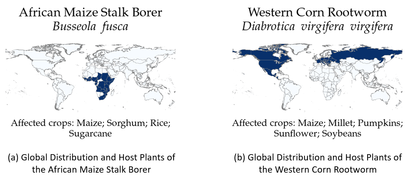
Notes: Each sub-figure displays the global distribution and host plant lists for the corresponding pest. The dark countries in the maps are ones in which the pest is known to be present. Data were collected from the Crop Pest Compendium (CPC) published by the Center for Agricultural Biosciences International (CABI).
We show that global innovation focuses systematically on the CPP threats of high-income countries. As one example, a CPP found in the US is, on average, mentioned in 57 agricultural patents filed globally since 2000, while a CPP not found in the US is mentioned in 11. This pattern is driven primarily by local bias–in all countries, a locally present CPP is 17 times more likely to be mentioned in a patent than a non-locally present CPP (Figure 2b). Since rich countries do more R&D, this local bias translates into an aggregate rich-world bias in the ecological conditions that receive the most attention.
Ecological differences impede technology diffusion
Motivated by these results, we develop a data set of CPP Mismatch for all crops and countries. This measure captures the differences in the set of CPP threats for each crop between each country and the country where most technology development for that crop takes place. We then study how disparities in the focus of technology influence global technology diffusion and adoption. In particular, does ecological mismatch with the centres of crop technology development limit technology transfer?
As our main proxy for technology diffusion, we measure the development and international transfer of agricultural biotechnology using data on all instances of intellectual property protection for uniquely identified seed varieties around the world. We constructed this data set using proprietary data from the International Union for the Protection of New Varieties of Plants (UPOV), the organisation tasked with overseeing the global implementation of intellectual property protection for agricultural biotechnology.
Figure 2 : The average number of patents per CPP for CPPs present in the US and CPPs not present in the US
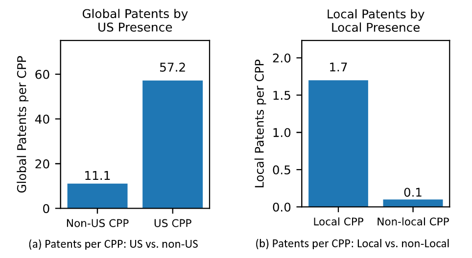
Notes: Figure 2(a) reports the average number of patents per CPP for CPPs present in the US and CPPs not present in the US. Figure 2(b) reports the average number of patents per CPP by inventors in a given country when the CPP is also present in the country and the average number of patents when the CPP is not present in the country. CPPs were linked to the full set of biological and chemical agricultural patents by searching for the CPP scientific name in all patent titles and abstracts.
Ecological mismatch substantially inhibits technology transfer: for the median value of CPP mismatch, technology diffusion is reduced by 44%. These results convey that the direction of innovation in research-intensive countries generates technology mismatch – gaps between what technology is designed to do and what it needs to do – which inhibits technology diffusion around the world.
This effect is equally strong for destination countries at all parts of the income distribution, suggesting that, even in the poorest regions, when mismatch is low technology does flow. To make this point even more concrete, we focus on the decisions of smallholder farmers in Africa. Using data from the World Bank’s Integrated Survey of Agriculture from eight African countries, we find that ecological mismatch with frontier innovators predicts significantly less self-reported use of improved seed varieties. While a large body of work has focused on how farmers’ constraints shapes their input adoption, these findings show that another important factor is the nature of technology, which is shaped not by farmers themselves but by innovating firms thousands of miles away.
Technology mismatch as a source of productivity differences
We next study how technology mismatch affects global agricultural productivity. We first find that ecological mismatch severely reduces agricultural production. Across countries and crops, a one standard-deviation change in ecological mismatch predicts a 0.51 standard-deviation reduction in crop-specific output (Figure 3a). The relationship is similar if we focus within two large agricultural economies, Brazil and India, where we find that mismatch lowers crop-specific production in more ecologically mismatched state-crop pairs (Figure 3b).
Figure 3: Ecological mismatch and output
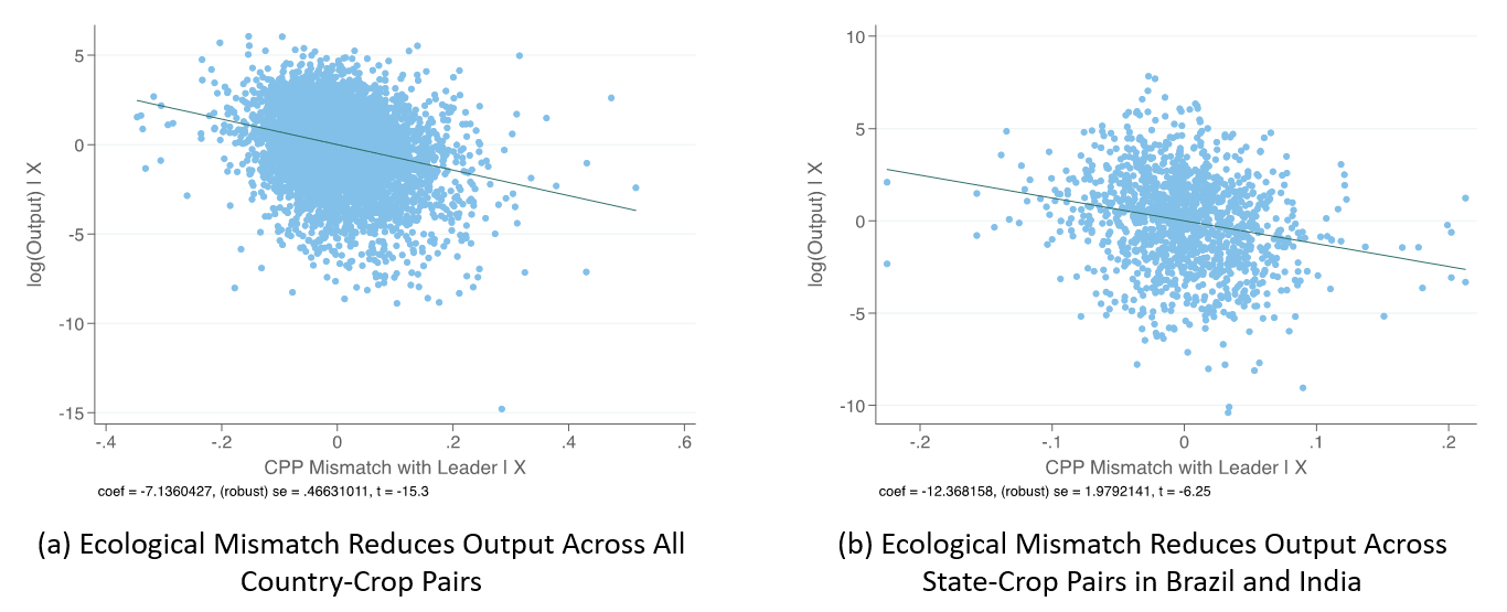
Notes: Figure 3(a) reports a partial correlation plot between log output and CPP mismatch at the crop-by-country level (p<0.01), with crop and country fixed effects partialled out. Figure 3(b) reports a partial correlation plot between log output and CPP mismatch at the crop-by-state level for Brazil and India (p<0.01), with crop-by-country and state fixed effects partialled out.
We combine our empirical estimates with an economic model of global production and directed innovation to quantify how technology mismatch, as we measure it, affects the global distribution of agricultural productivity. Compared to a world with no mismatch, in which research was equally focused on all pest and pathogen threats, agricultural productivity is 58% lower and disparities across countries are 15% higher. Large parts of Africa are most negatively affected.
Broader scope: Future policy, emerging market R&D, and climate change
Our paper focuses on the current state of global innovation and ecological mismatch and shows how the rich-world focus of technology can explain a large share of global agricultural productivity differences. However, several global changes in innovation and in the environment might alter the story in important ways.
One potential driver of future technology mismatch is policy change. The main proposed policy solution to technology mismatch is coordinated investment in R&D outside rich countries. This was a major motivation behind the Green Revolution of the 1960s and 70s, during which international organisations invested substantially in breeding research in specific tropical countries. While the Green Revolution led to dramatic productivity growth in large parts of the world, we show that the productivity benefits were limited in countries with higher ecological mismatch from the specific centres of Green Revolution breeding. For example, large parts of Africa saw little benefit from the Green Revolution because their ecological conditions are distinct from the dominant Green Revolution research centres in India, Mexico, and the Philippines.
More recently, there have been calls for a “Second Green Revolution” that also benefits parts of the world left behind by the first Green Revolution. Using our data, we can identify the locations of crop-specific breeding that could generate new technology with the lowest possible ecological mismatch to the least productive parts of the world.
These results suggest large global benefits to R&D targeted toward several crop-specific environments in sub-Saharan Africa and South Asia, including Nigeria, Tanzania, Zimbabwe, the DRC, Ghana, India, and Pakistan. Rigorous modelling of technology mismatch should be at the centre of any global R&D policy.
A second potential driver of future technology mismatch is the rise of emerging market R&D, most notably in Brazil, Russia, India and China (the BRICs). We find potentially large global benefits from this re-shuffling of technological leadership due to the fact that BRIC ecology is, on average, more similar to low- and middle-income countries than is the current set of technological leaders.
A final potential driver of future technological mismatch is climate change. In other work, we have shown that innovating firms have dramatically shifted their focus toward developing new seed varieties for the crops currently most affected by heat in the US (Moscona and Sastry forthcoming). However, we find no evidence of similar efforts targeting the set of crops that is most affected by heat in low-income countries. This cross-crop mismatch in climate damage layers on top of the ecological mismatch that we describe above, which impedes technology diffusion for a single crop across environments.
At the same time, as the world gets warmer and CPPs migrate poleward (Bebber et al. 2013), high-income countries might inherit some of the CPP threats that currently reside only in low-income countries. This could mean that high- and low-income countries face a more common set of ecological threats, and rich countries face increased incentives to develop technologies to combat threats that had previously been limited to poor countries. We leave a full appraisal of how climate change shifts global ecology, technology mismatch, and productivity to future work.
Access to Seeds Foundation (2019), Access to Seeds Index: 2019 Synthesis Report , Accessed from: https://www.accesstoseeds.org/media/publications/.
Acemoglu, D and F Zilibotti (2001), “Productivity differences”, The Quarterly Journal of Economics 116(2): 563-606.
Bebber, D P, M A Ramotowski and S J Gurr (2013), “Crop pests and pathogens move polewards in a warming world”, Nature climate change 3(11): 985-988.
Caselli, F (2005), “Accounting for cross-country income differences”, Handbook of economic growth 1:679-741.
Dong, O X and P C Ronald (2019), “Genetic engineering for disease resistance in plants: recent progress and future perspectives”, Plant physiology 180(1): 26-38.
Fuglie, K (2016), “The growing role of the private sector in agricultural research and development world-wide”, Global food security 10: 29-38.
McMullen, N (1987), Seeds and world agricultural progress , National Planning Association.
Moscona, J and K A Sastry (2022), “Inappropriate technology: Evidence from global agriculture”, Working Paper, Available from: https://papers.ssrn.com/sol3/papers.cfm?abstract_id=3886019.
Moscona, J and K A Sastry (forthcoming), “Does Directed Innovation Mitigate Climate Damage? Evidence from US Agriculture”, The Quarterly Journal of Economics , Available from: https://doi.org/10.1093/qje/qjac039.
Oerke, E C & H W Dehne (2004), “Safeguarding production—losses in major crops and the role of crop protection”, Crop Protection 23(4): 275-285.
Stewart, F (1978), Technology and Underdevelopment , London: MacMillan
Information
- Author Services
Initiatives
You are accessing a machine-readable page. In order to be human-readable, please install an RSS reader.
All articles published by MDPI are made immediately available worldwide under an open access license. No special permission is required to reuse all or part of the article published by MDPI, including figures and tables. For articles published under an open access Creative Common CC BY license, any part of the article may be reused without permission provided that the original article is clearly cited. For more information, please refer to https://www.mdpi.com/openaccess .
Feature papers represent the most advanced research with significant potential for high impact in the field. A Feature Paper should be a substantial original Article that involves several techniques or approaches, provides an outlook for future research directions and describes possible research applications.
Feature papers are submitted upon individual invitation or recommendation by the scientific editors and must receive positive feedback from the reviewers.
Editor’s Choice articles are based on recommendations by the scientific editors of MDPI journals from around the world. Editors select a small number of articles recently published in the journal that they believe will be particularly interesting to readers, or important in the respective research area. The aim is to provide a snapshot of some of the most exciting work published in the various research areas of the journal.
Original Submission Date Received: .
- Active Journals
- Find a Journal
- Journal Proposal
- Proceedings Series
- For Authors
- For Reviewers
- For Editors
- For Librarians
- For Publishers
- For Societies
- For Conference Organizers
- Open Access Policy
- Institutional Open Access Program
- Special Issues Guidelines
- Editorial Process
- Research and Publication Ethics
- Article Processing Charges
- Testimonials
- Preprints.org
- SciProfiles
- Encyclopedia
Article Menu

- Subscribe SciFeed
- Recommended Articles
- Google Scholar
- on Google Scholar
- Table of Contents
Find support for a specific problem in the support section of our website.
Please let us know what you think of our products and services.
Visit our dedicated information section to learn more about MDPI.
JSmol Viewer
Synergistic impacts of climate change and wildfires on agricultural sustainability—a greek case study.

1. Introduction
1.1. background to the study, 1.2. objectives of the study.
- To examine the effect of extreme weather events on agricultural sustainability in Europe.
- To evaluate the ecosystem disruption caused by climate change and its effect on agricultural sustainability in Europe.
- To evaluate wildlife habitat alteration by wildfires and its influence on agricultural sustainability in Europe.
- To examine the influence of wildfire smoke on the general sustainability of agriculture across Europe.
1.3. Literature Review
1.3.1. extreme weather events, 1.3.2. ecosystem disruption caused by climate change, 1.3.3. habitat alteration by wildfires, 1.3.4. wildfire smoke, 1.3.5. climate change and sustainability of agriculture across europe, 1.4. research questions.
- What is the effect of extreme weather events on agricultural sustainability in Europe?
- How does the ecosystem disruption caused by climate change affect agricultural sustainability in Europe?
- How does wildlife habitat alteration by wildfires influence agricultural sustainability in Europe?
- What is the influence of wildfire smoke on the general sustainability of agriculture across Europe?
1.5. Research Hypotheses
2. methodology, 2.1. research design, 2.2. target population, 2.3. sample size, 2.4. data collection, 2.5. data analysis, 3.1. descriptive results, 3.2. regression analysis, 4. discussion, 5. conclusions, limitations and areas for future research, author contributions, data availability statement, acknowledgments, conflicts of interest.
- Jhariya, M.K.; Raj, A. Effects of Wildfires on Flora, Fauna and Physico-Chemical Properties of Soil-An Overview. J. Appl. Nat. Sci. 2014 , 6 , 887–897. [ Google Scholar ] [ CrossRef ]
- Marlier, M.E.; Brenner, K.I.; Liu, J.C.; Mickley, L.J.; Raby, S.; James, E.; Ahmadov, R.; Riden, H. Exposure of Agricultural Workers in California to Wildfire Smoke under Past and Future Climate Conditions. Environ. Res. Lett. 2022 , 17 , 094045. [ Google Scholar ] [ CrossRef ]
- Meier, S.; Elliott, R.J.R.; Strobl, E. The Regional Economic Impact of Wildfires: Evidence from Southern Europe. J. Environ. Econ. Manage. 2023 , 118 , 102787. [ Google Scholar ] [ CrossRef ]
- Masoom, A.; Fountoulakis, I.; Kazadzis, S.; Raptis, I.P.; Kampouri, A.; Psiloglou, B.E.; Kouklaki, D.; Papachristopoulou, K.; Marinou, E.; Solomos, S.; et al. Investigation of the Effects of the Greek Extreme Wildfires of August 2021 on Air Quality and Spectral Solar Irradiance. Atmos. Chem. Phys. 2023 , 23 , 8487–8514. [ Google Scholar ] [ CrossRef ]
- Sutton, W.R.; Block, R.I.; Srivastava, J. Adaptation to Climate Change in Europe and Central Asia Agriculture ; World Bank: Washington, DC, USA, 2009; pp. 1–61. [ Google Scholar ] [ CrossRef ]
- Gitz, V.; Meybeck, A.; Lipper, L. Climate Change and Food Security: Risks and Responses ; FAO: Rome, Italy, 2015; ISBN 978-92-5-108998-9. [ Google Scholar ]
- Mouat, D.; Lancaster, J.; El-Bagouri, I.; Santibañez, F. Opportunities for Synergy Among the Environmental Conventions: Results of National and Local Level Workshops ; Secretariat of the United Nations Convention to Combat Desertification (UNCCD): Bonn, Germany, 2006; ISBN 9789295043152. [ Google Scholar ]
- Do, V.Q.; Phung, M.L.; Truong, D.T.; Pham, T.T.T.; Dang, V.T.; Nguyen, T.K. The Impact of Extreme Events and Climate Change on Agricultural and Fishery Enterprises in Central Vietnam. Sustainability 2021 , 13 , 7121. [ Google Scholar ] [ CrossRef ]
- Kim, C. The Impact of Climate Change on the Agricultural Sector: Implications of the Agro-Industry for Low Carbon, Green Growth Strategy and Roadmap for the East Asian Region. In Low Carbon Green Growth Roadmap Asia and the Pacific ; Economic and Social Commission for Asia and the Pacific (ESCAP): Bangkok, Thailand, 2012; pp. 1–51. [ Google Scholar ]
- Schipper, E.L.F.; Revi, A.; Preston, B.L.; Carr, E.R.; Eriksen, S.H.; Fernández-Carril, L.R.; Glavovic, B.; Hilmi, N.J.M.; Ley, D.; Mukerji, R.; et al. Summary for Policymakers. In Climate Change 2022—Impacts, Adaptation and Vulnerability ; Pörtner, H.-O., Roberts, D.C., Tignor, M., Poloczanska, E.S., Mintenbeck, K., Alegría, A., Craig, M., Langsdorf, S., Löschke, S., Möller, V., et al., Eds.; Cambridge University Press: New York, NY, USA, 2023; pp. 3–34. [ Google Scholar ]
- Stougiannidou, D.; Zafeiriou, E.; Raftoyannis, Y. Forest Fires in Greece and Their Economic Impacts on Agriculture. KnE Soc. Sci. 2020 , 54–70. [ Google Scholar ] [ CrossRef ]
- Furtak, K.; Wolińska, A. The Impact of Extreme Weather Events as a Consequence of Climate Change on the Soil Moisture and on the Quality of the Soil Environment and Agriculture—A Review. Catena 2023 , 231 , 107378. [ Google Scholar ] [ CrossRef ]
- Kumar, L.; Chhogyel, N.; Gopalakrishnan, T.; Hasan, M.K.; Jayasinghe, S.L.; Kariyawasam, C.S.; Kogo, B.K.; Ratnayake, S. Climate Change and Future of Agri-Food Production ; Elsevier Inc.: Amsterdam, The Netherlands, 2021; ISBN 9780323910019. [ Google Scholar ]
- Bednar-Friedl, B.; Biesbroek, R.; Schmidt, D.N.; Alexander, P.; Børsheim, K.Y.; Carnicer, J.; Georgopoulou, E.; Haasnoot, M.; Cozannet, G.L.; Lionello, P.; et al. Europe. In Climate Change 2022—Impacts, Adaptation and Vulnerability: Working Group II Contribution to the Sixth Assessment Report of the Intergovernmental Panel on Climate Change ; Pörtner, H.-O., Roberts, D.C., Tignor, M., Poloczanska, E.S., Mintenbeck, K., Alegría, A., Craig, M., Langsdorf, S., Löschke, S., Möller, V., et al., Eds.; Cambridge University Press: New York, NY, USA, 2023; pp. 1817–1928. ISBN 9781009325837. [ Google Scholar ]
- Khan, N.; Ma, J.; Zhang, H.; Zhang, S. Climate Change Impact on Sustainable Agricultural Growth: Insights from Rural Areas. Atmosphere 2023 , 14 , 1194. [ Google Scholar ] [ CrossRef ]
- Cittadino, F.; Meier, A.; Bertuzzi, N.; Felber, A.T.; Librera, T. Best Practices: Climate Change Policy Integration at the Subnational Level in Italy and Austria ; Eurac Research: Bolzano, Italy, 2022. [ Google Scholar ]
- Ayanlade, A.; Oluwaranti, A.; Ayanlade, O.S.; Borderon, M.; Sterly, H.; Sakdapolrak, P.; Jegede, M.O.; Weldemariam, L.F.; Ayinde, A.F.O. Extreme Climate Events in Sub-Saharan Africa: A Call for Improving Agricultural Technology Transfer to Enhance Adaptive Capacity. Clim. Serv. 2022 , 27 , 100311. [ Google Scholar ] [ CrossRef ]
- Bojar, W.; Knopik, L.; Żarski, J.; Sławiński, C.; Baranowski, P.; Żarski, W. Impact of Extreme Climate Changes on the Predicted Crops in Poland. Acta Agrophysica 2014 , 21 , 415–431. [ Google Scholar ]
- Loizou, E.; Chatzitheodoridis, F.; Michailidis, A.; Tsakiri, M.; Theodossiou, G. Linkages of the Energy Sector in the Greek Economy: An Input-Output Approach. Int. J. Energy Sect. Manag. 2015 , 9 , 393–411. [ Google Scholar ] [ CrossRef ]
- Kulkarni, C.; Finsinger, W.; Anand, P.; Nogué, S.; Bhagwat, S.A. Synergistic Impacts of Anthropogenic Fires and Aridity on Plant Diversity in the Western Ghats: Implications for Management of Ancient Social-Ecological Systems. J. Environ. Manag. 2021 , 283 , 111957. [ Google Scholar ] [ CrossRef ] [ PubMed ]
- WMO United in Science 2023. Sustainable Development Edition. A Multi-Organization High-Level Compilation of the Latest Weather-, Climateand Water-Related Sciences and Services for Sustainable Development ; World Meteorological Organization (WMO): Geneva, Switzerland, 2023; pp. 1–48. [ Google Scholar ]
- Malhi, G.S.; Kaur, M.; Kaushik, P. Impact of Climate Change on Agriculture and Its Mitigation Strategies: A Review. Sustainability 2021 , 13 , 1318. [ Google Scholar ] [ CrossRef ]
- Ciscar, J.C.; Ibarreta, D.; Soria, A.; Dosio, A.; Toreti, A.; Ceglar, A.; Fumagalli, D.; Dentener, F.; Lecerf, R.; Zucchini, A. Climate Impacts in Europe: Final Report of the JRC PESETA III Project ; JRC Science for Policy Report EUR 29427 EN; Publications Office of the European Union: Luxembourg, 2018; ISBN 978-92-79-97218-8. [ Google Scholar ]
- Tekalign, W.; Kebede, Y.; Sodo, W. Impacts of Wildfire and Prescribed Fire on Wildlife and Habitats: A Review. J. Nat. Sci. Res. 2016 , 6 , 15–27. [ Google Scholar ]
- Egger, C.; Mayer, A.; Bertsch-Hörmann, B.; Plutzar, C.; Schindler, S.; Tramberend, P.; Haberl, H.; Gaube, V. Effects of Extreme Events on Land-Use-Related Decisions of Farmers in Eastern Austria: The Role of Learning. Agron. Sustain. Dev. 2023 , 43 , 39. [ Google Scholar ] [ CrossRef ]
- Jaramillo, L.; Close; Cebotari, A.; Diallo, Y.; Gupta, R.; Koshima, Y.; International Monetary Fund; Kularatne, C.; Lee, J.D.; Rehman, S.; et al. Climate Challenges in Fragile and Conflict-Affected States. Staff Clim. Notes 2023 , 2023 , 1. [ Google Scholar ] [ CrossRef ]
- Yakupoğlu, T.; Dindaroğlu, T.; Rodrigo-Comino, J.; Cerdà, A. Stubble Burning and Wildfires in Turkey Considering the Sustainable Development Goals of the United Nations. Eurasian J. Soil Sci. 2022 , 11 , 66–76. [ Google Scholar ] [ CrossRef ]
- Clarke, B.; Otto, F.; Stuart-Smith, R.; Harrington, L. Extreme Weather Impacts of Climate Change: An Attribution Perspective. Environ. Res. Clim. 2022 , 1 , 12001. [ Google Scholar ] [ CrossRef ]
- Zscheischler, J.; Martius, O.; Westra, S.; Bevacqua, E.; Raymond, C.; Horton, R.M.; van den Hurk, B.; AghaKouchak, A.; Jézéquel, A.; Mahecha, M.D.; et al. A Typology of Compound Weather and Climate Events. Nat. Rev. Earth Environ. 2020 , 1 , 333–347. [ Google Scholar ] [ CrossRef ]
- Weilnhammer, V.; Schmid, J.; Mittermeier, I.; Schreiber, F.; Jiang, L.; Pastuhovic, V.; Herr, C.; Heinze, S. Extreme Weather Events in Europe and Their Health Consequences—A Systematic Review. Int. J. Hyg. Environ. Health 2021 , 233 , 113688. [ Google Scholar ] [ CrossRef ]
- Beillouin, D.; Schauberger, B.; Bastos, A.; Ciais, P.; Makowski, D. Impact of Extreme Weather Conditions on European Crop Production in 2018. Philos. Trans. R. Soc. B Biol. Sci. 2020 , 375 , 20190510. [ Google Scholar ] [ CrossRef ] [ PubMed ]
- Weaver, S.M.; Guinan, P.E.; Semenova, I.G.; Aloysius, N.; Lupo, A.R.; Hunt, S. A Case Study of Drought during Summer 2022: A Large-Scale Analyzed Comparison of Dry and Moist Summers in the Midwest USA. Atmosphere 2023 , 14 , 1448. [ Google Scholar ] [ CrossRef ]
- Mao, H.; Zhang, X.; Fu, Y. Farmers’ Adaptation to Extreme Weather: Evidence from Rural China. Res. Sq. 2022 . [ Google Scholar ] [ CrossRef ]
- Planisich, A.; Utsumi, S.A.; Larripa, M.; Galli, J.R. Grazing of Cover Crops in Integrated Crop-Livestock Systems. Animal 2021 , 15 , 100054. [ Google Scholar ] [ CrossRef ] [ PubMed ]
- Brempong, M.B.; Amankwaa-Yeboah, P.; Yeboah, S.; Owusu Danquah, E.; Agyeman, K.; Keteku, A.K.; Addo-Danso, A.; Adomako, J. Soil and Water Conservation Measures to Adapt Cropping Systems to Climate Change Facilitated Water Stresses in Africa. Front. Sustain. Food Syst. 2023 , 6 , 1091665. [ Google Scholar ] [ CrossRef ]
- Savari, M.; Eskandari Damaneh, H.; Damaneh, H.E. Factors Influencing Farmers’ Management Behaviors toward Coping with Drought: Evidence from Iran. J. Environ. Plan. Manag. 2021 , 64 , 2021–2046. [ Google Scholar ] [ CrossRef ]
- Holleman, C.; Rembold, F.; Crespo, O.; Conti, V. The Impact of Climate Variability and Extremes on Agriculture and Food Security—an Analysis of the Evidence and Case Studies. Background Paper for the State of Food Security and Nutrition in the World 2018 ; FAO Agricultural Development Economics Technical Study No. 4; FAO: Rome, Italy, 2020. [ Google Scholar ] [ CrossRef ]
- Muluneh, M.G. Impact of Climate Change on Biodiversity and Food Security: A Global Perspective—A Review Article. Agric. Food Secur. 2021 , 10 , 1–25. [ Google Scholar ] [ CrossRef ]
- Radović, V.; Pejanović, R.; Marinčić, D. Extreme Weather and Climatic Events on Agriculture as a Risk of Sustainable Development. Ekon. Poljopr. 2015 , 62 , 181–191. [ Google Scholar ] [ CrossRef ]
- Gornall, J.; Betts, R.; Burke, E.; Clark, R.; Camp, J.; Willett, K.; Wiltshire, A. Implications of Climate Change for Agricultural Productivity in the Early Twenty-First Century. Philos. Trans. R. Soc. B Biol. Sci. 2010 , 365 , 2973–2989. [ Google Scholar ] [ CrossRef ]
- Shah, W.U.H.; Lu, Y.; Liu, J.; Rehman, A.; Yasmeen, R. The Impact of Climate Change and Production Technology Heterogeneity on China’s Agricultural Total Factor Productivity and Production Efficiency. Sci. Total Environ. 2024 , 907 , 168027. [ Google Scholar ] [ CrossRef ]
- Kalogiannidis, S.; Chatzitheodoridis, F.; Kalfas, D.; Patitsa, C.; Papagrigoriou, A. Socio-Psychological, Economic and Environmental Effects of Forest Fires. Fire 2023 , 6 , 280. [ Google Scholar ] [ CrossRef ]
- Chatzitheodoridis, F.; Kontogeorgos, A.; Liltsi, P.; Apostolidou, I.; Michailidis, A.; Loizou, E. Women’s Cooperatives in Less Favored and Mountainous Areas under Economic Instability. Agric. Econ. Rev. 2016 , 17 , 63–79. [ Google Scholar ]
- Zharkov, D.; Nizamutdinov, T.; Dubovikoff, D.; Abakumov, E.; Pospelova, A. Navigating Agricultural Expansion in Harsh Conditions in Russia: Balancing Development with Insect Protection in the Era of Pesticides. Insects 2023 , 14 , 557. [ Google Scholar ] [ CrossRef ]
- Naqvi, S.A.H.; Rehman, A.U.; Chohan, S.; Umar, U.U.D.; Mehmood, Y.; Mustafa, G.; Nazir, W.; Hasnain, A. Sustainable Development in Agriculture Beyond the Notion of Minimizing Environmental Impacts. In Disaster Risk Reduction in Agriculture ; Ahmed, M., Ahmad, S., Eds.; Springer Nature: Singapore, 2023; pp. 147–168. ISBN 978-981-99-1763-1. [ Google Scholar ]
- Cogato, A.; Meggio, F.; Migliorati, M.D.A.; Marinello, F. Extreme Weather Events in Agriculture: A Systematic Review. Sustainability 2019 , 11 , 2547. [ Google Scholar ] [ CrossRef ]
- Habib-ur-Rahman, M.; Ahmad, A.; Raza, A.; Hasnain, M.U.; Alharby, H.F.; Alzahrani, Y.M.; Bamagoos, A.A.; Hakeem, K.R.; Ahmad, S.; Nasim, W.; et al. Impact of Climate Change on Agricultural Production; Issues, Challenges, and Opportunities in Asia. Front. Plant Sci. 2022 , 13 , 925548. [ Google Scholar ] [ CrossRef ] [ PubMed ]
- Semeraro, T.; Scarano, A.; Leggieri, A.; Calisi, A.; Caroli, M.D. Impact of Climate Change on Agroecosystems and Potential Adaptation Strategies. Land 2023 , 12 , 1117. [ Google Scholar ] [ CrossRef ]
- Kertész, M.; Aszalós, R.; Lengyel, A.; Ónodi, G. Synergistic Effects of the Components of Global Change: Increased Vegetation Dynamics in Open, Forest-Steppe Grasslands Driven by Wildfires and Year-to-Year Precipitation Differences. PLoS ONE 2017 , 12 , 1–11. [ Google Scholar ] [ CrossRef ]
- Liu, Z.; Zhao, M.; Zhang, H.; Ren, T.; Liu, C.; He, N. Divergent Response and Adaptation of Specific Leaf Area to Environmental Change at Different Spatio-Temporal Scales Jointly Improve Plant Survival. Glob. Chang. Biol. 2023 , 29 , 1144–1159. [ Google Scholar ] [ CrossRef ]
- Quandt, A.; Neufeldt, H.; Gorman, K. Climate Change Adaptation through Agroforestry: Opportunities and Gaps. Curr. Opin. Environ. Sustain. 2023 , 60 , 101244. [ Google Scholar ] [ CrossRef ]
- Araújo, M.B.; Anderson, R.P.; Márcia Barbosa, A.; Beale, C.M.; Dormann, C.F.; Early, R.; Garcia, R.A.; Guisan, A.; Maiorano, L.; Naimi, B.; et al. Standards for Distribution Models in Biodiversity Assessments. Sci. Adv. 2024 , 5 , eaat4858. [ Google Scholar ] [ CrossRef ]
- Heberling, J.M.; Miller, J.T.; Noesgaard, D.; Weingart, S.B.; Schigel, D. Data Integration Enables Global Biodiversity Synthesis. Proc. Natl. Acad. Sci. USA 2021 , 118 , e2018093118. [ Google Scholar ] [ CrossRef ] [ PubMed ]
- Bachmann, J.C.; Jansen van Rensburg, A.; Cortazar-Chinarro, M.; Laurila, A.; Van Buskirk, J. Gene Flow Limits Adaptation along Steep Environmental Gradients. Am. Nat. 2020 , 195 , E67–E86. [ Google Scholar ] [ CrossRef ] [ PubMed ]
- D’Evelyn, S.M.; Jung, J.; Alvarado, E.; Baumgartner, J.; Caligiuri, P.; Hagmann, R.K.; Henderson, S.B.; Hessburg, P.F.; Hopkins, S.; Kasner, E.J.; et al. Wildfire, Smoke Exposure, Human Health, and Environmental Justice Need to Be Integrated into Forest Restoration and Management. Curr. Environ. Health Rep. 2022 , 9 , 366–385. [ Google Scholar ] [ CrossRef ]
- Annappa; Bhavya; Kasturappa, G.; Kumar, U. Climate Change’s Threat to Agriculture: Impacts, Challenges and Strategies for a Sustainable Future ; AkiNik Publications: New Delhi, India, 2023. [ Google Scholar ]
- Agbeshie, A.A.; Abugre, S.; Atta-Darkwa, T.; Awuah, R. A Review of the Effects of Forest Fire on Soil Properties. J. For. Res. 2022 , 33 , 1419–1441. [ Google Scholar ] [ CrossRef ]
- Antwi-Agyei, P.; Atta-Aidoo, J.; Asare-Nuamah, P.; Stringer, L.C.; Antwi, K. Trade-Offs, Synergies and Acceptability of Climate Smart Agricultural Practices by Smallholder Farmers in Rural Ghana. Int. J. Agric. Sustain. 2023 , 21 , 2193439. [ Google Scholar ] [ CrossRef ]
- Ewusie, Y. Elements of Tropical Ecology ; Heinemann Educational Books: Portsmouth, NH, USA, 1980; ISBN 0435937006. [ Google Scholar ]
- Bowman, D.M.J.S.; Kolden, C.A.; Abatzoglou, J.T.; Johnston, F.H.; van der Werf, G.R.; Flannigan, M. Vegetation Fires in the Anthropocene. Nat. Rev. Earth Environ. 2020 , 1 , 500–515. [ Google Scholar ] [ CrossRef ]
- Garcês, A.; Pires, I. The Hell of Wildfires: The Impact on Wildlife and Its Conservation and the Role of the Veterinarian. Conservation 2023 , 3 , 96–108. [ Google Scholar ] [ CrossRef ]
- Certini, G.; Moya, D.; Lucas-Borja, M.E.; Mastrolonardo, G. The Impact of Fire on Soil-Dwelling Biota: A Review. For. Ecol. Manag. 2021 , 488 , 118989. [ Google Scholar ] [ CrossRef ]
- Gutsche, R.E.; Pinto, J. Covering Synergistic Effects of Climate Change: Global Challenges for Journalism. J. Pract. 2022 , 16 , 237–243. [ Google Scholar ] [ CrossRef ]
- Kalfas, D.; Kalogiannidis, S.; Chatzitheodoridis, F.; Margaritis, N. The Other Side of Fire in a Changing Environment: Evidence from a Mediterranean Country. Fire 2024 , 7 , 36. [ Google Scholar ] [ CrossRef ]
- Mahdi, S.S. Climate Change and Agriculture in India: Impact and Adaptation ; Springer: Cham, Switzerland, 2019; pp. 1–262. [ Google Scholar ] [ CrossRef ]
- Carnicer, J.; Alegria, A.; Giannakopoulos, C.; Di Giuseppe, F.; Karali, A.; Koutsias, N.; Lionello, P.; Parrington, M.; Vitolo, C. Global Warming Is Shifting the Relationships between Fire Weather and Realized Fire-Induced CO2 Emissions in Europe. Sci. Rep. 2022 , 12 , 10365. [ Google Scholar ] [ CrossRef ] [ PubMed ]
- Pellegrini, A.F.A.; Harden, J.; Georgiou, K.; Hemes, K.S.; Malhotra, A.; Nolan, C.J.; Jackson, R.B. Fire Effects on the Persistence of Soil Organic Matter and Long-Term Carbon Storage. Nat. Geosci. 2022 , 15 , 5–13. [ Google Scholar ] [ CrossRef ]
- Merino, A.; Fonturbel, M.T.; Fernández, C.; Chávez-Vergara, B.; García-Oliva, F.; Vega, J.A. Inferring Changes in Soil Organic Matter in Post-Wildfire Soil Burn Severity Levels in a Temperate Climate. Sci. Total Environ. 2018 , 627 , 622–632. [ Google Scholar ] [ CrossRef ] [ PubMed ]
- Ampaire, E.L.; Acosta, M.; Huyer, S.; Kigonya, R.; Muchunguzi, P.; Muna, R.; Jassogne, L. Gender in climate change, agriculture, and natural resource policies: Insights from East Africa. Clim. Chang. 2020 , 158. [ Google Scholar ] [ CrossRef ]
- Stavi, I. Wildfires in Grasslands and Shrublands: A Review of Impacts on Vegetation, Soil, Hydrology, and Geomorphology. Water 2019 , 11 , 1042. [ Google Scholar ] [ CrossRef ]
- Krueger, E.S.; Ochsner, T.E.; Levi, M.R.; Basara, J.B.; Snitker, G.J.; Wyatt, B.M. Grassland Productivity Estimates Informed by Soil Moisture Measurements: Statistical and Mechanistic Approaches. Agron. J. 2021 , 113 , 3498–3517. [ Google Scholar ] [ CrossRef ]
- Ashton, P.; Zhu, H. The Tropical-Subtropical Evergreen Forest Transition in East Asia: An Exploration. Plant Divers. 2020 , 42 , 255–280. [ Google Scholar ] [ CrossRef ]
- Arora, N.K. Impact of Climate Change on Agriculture Production and Its Sustainable Solutions. Environ. Sustain. 2019 , 2 , 95–96. [ Google Scholar ] [ CrossRef ]
- Hemes, K.S.; Verfaillie, J.; Baldocchi, D.D. Wildfire-Smoke Aerosols Lead to Increased Light Use Efficiency Among Agricultural and Restored Wetland Land Uses in California’s Central Valley. J. Geophys. Res. Biogeosciences 2020 , 125 , e2019JG005380. [ Google Scholar ] [ CrossRef ]
- Etumnu, C.; Wang, T.; Jin, H.; Sieverding, H.L.; Ulrich-Schad, J.D.; Clay, D. Understanding Farmers’ Perception of Extreme Weather Events and Adaptive Measures. Clim. Risk Manag. 2023 , 40 , 100494. [ Google Scholar ] [ CrossRef ]
- Devot, A.; Royer, L.; Caron Giauffret, E.; Ayral, V.; Deryng, D.; Arvis, B.; Giraud, L.; Roullard, J. Research for AGRI Committee—The Impact of Extreme Climate Events on Agriculture Production in the EU ; European Parliament, Policy Department for Structural and Cohesion Policies: Brussels, Belgium, 2023. [ Google Scholar ]
- Angelakιs, A.N.; Zaccaria, D.; Krasilnikoff, J.; Salgot, M.; Bazza, M.; Roccaro, P.; Jimenez, B.; Kumar, A.; Yinghua, W.; Baba, A.; et al. Irrigation of World Agricultural Lands: Evolution through the Millennia. Water 2020 , 12 , 1285. [ Google Scholar ] [ CrossRef ]
- Clark, D.A. Sources or Sinks? The Responses of Tropical Forests to Current and Future Climate and Atmospheric Composition. Philos. Trans. R. Soc. B Biol. Sci. 2004 , 359 , 477–491. [ Google Scholar ] [ CrossRef ] [ PubMed ]
- Berninger, K.; Lager, F.; Holm Tara, B.; Tynkkynen, O.; Klein, R.J.T.; Aall, C.; Dristig, A.; Määttä, H.; Perrels, A. Nordic Perspectives on Transboundary Climate Risk: Current Knowledge and Pathways for Action ; Nordic Council of Ministers: Copenhagen, Denmark, 2022. [ Google Scholar ]
- Kalfas, D.G.; Zagkas, D.T.; Raptis, D.I.; Zagkas, T.D. The Multifunctionality of the Natural Environment through the Basic Ecosystem Services in the Florina Region, Greece. Int. J. Sustain. Dev. World Ecol. 2019 , 26 , 57–68. [ Google Scholar ] [ CrossRef ]
- Kalfas, D.G.; Zagkas, D.T.; Dragozi, E.I.; Melfou, K.Κ. An Approach of Landsenses Ecology and Landsenseology in Greece. Int. J. Sustain. Dev. World Ecol. 2021 , 28 , 677–692. [ Google Scholar ] [ CrossRef ]
- Shivanna, K.R. The Plight of Bees and Other Pollinators, and Its Consequences on Crop Productivity. Resonance 2022 , 27 , 785–799. [ Google Scholar ] [ CrossRef ]
- Chatzitheodoridis, F.; Michailidis, A.; Theodosiou, G.; Loizou, E. Local Cooperation: A Dynamic Force for Endogenous Rural Development BT—Balkan and Eastern European Countries in the Midst of the Global Economic Crisis. In Balkan and Eastern European Countries in the Midst of the Global Economic Crisis ; Karasavvoglou, A., Polychronidou, P., Eds.; Physica-Verlag HD: Heidelberg, Germany, 2013; pp. 121–132. ISBN 978-3-7908-2873-3. [ Google Scholar ]
- Creswell, J.W.; Creswell, J.D. Research Design: Qualitative, Quantitative, and Mixed Methods Approaches , 5th ed.; Sage Publications: Los Angeles, CA, USA, 2018; ISBN 1506386717. [ Google Scholar ]
- Bryman, A. Social Research Methods , 5th ed.; Oxford University Press: London, UK, 2016; ISBN 0199689458. [ Google Scholar ]
- Krejcie, R.V.; Morgan, D.W. Determining Sample Size for Research Activities. Educ. Psychol. Meas. 1970 , 30 , 607–610. [ Google Scholar ] [ CrossRef ]
- Kalogiannidis, S.; Kalfas, D.; Giannarakis, G.; Paschalidou, M. Integration of Water Resources Management Strategies in Land Use Planning towards Environmental Conservation. Sustainability 2023 , 15 , 15242. [ Google Scholar ] [ CrossRef ]
- Kalogiannidis, S.; Kalfas, D.; Loizou, E.; Chatzitheodoridis, F. Forestry Bioeconomy Contribution on Socioeconomic Development: Evidence from Greece. Land 2022 , 11 , 2139. [ Google Scholar ] [ CrossRef ]
Click here to enlarge figure
| N | n | N | n | N | n |
|---|---|---|---|---|---|
| 10 | 10 | 220 | 140 | 1200 | 291 |
| 15 | 14 | 230 | 144 | 1300 | 297 |
| 20 | 19 | 240 | 148 | 1400 | 302 |
| 25 | 24 | 250 | 152 | 1500 | 306 |
| 30 | 28 | 260 | 155 | 1600 | 310 |
| 35 | 32 | 270 | 159 | 1700 | 313 |
| 40 | 36 | 280 | 162 | 1800 | 317 |
| 45 | 40 | 290 | 165 | 1900 | 320 |
| 50 | 44 | 300 | 169 | 2000 | 322 |
| 55 | 48 | 320 | 175 | 2800 | 338 |
| 60 | 52 | 340 | 181 | 3000 | 341 |
| 65 | 56 | 360 | 186 | 3500 | 346 |
| 70 | 59 | 380 | 191 | 4000 | 351 |
| 75 | 63 | 400 | 196 | 4500 | 354 |
| 80 | 66 | 420 | 201 | 5000 | 357 |
| 85 | 70 | 440 | 205 | 6000 | 361 |
| 90 | 73 | 460 | 210 | 7000 | 364 |
| 95 | 76 | 480 | 214 | 8000 | 367 |
| 100 | 80 | 500 | 217 | 9000 | 368 |
| 110 | 86 | 550 | 226 | 10,000 | 370 |
| 120 | 92 | 600 | 234 | 15,000 | 375 |
| 130 | 97 | 650 | 242 | 20,000 | 377 |
| 140 | 103 | 700 | 248 | 30,000 | 379 |
| 150 | 108 | 750 | 254 | 40,000 | 380 |
| 160 | 113 | 800 | 260 | 50,000 | 381 |
| 170 | 118 | 850 | 265 | 75,000 | 382 |
| 180 | 123 | 900 | 269 | 1,000,000 | 384 |
| Characteristic | Frequency | Percentage (%) |
|---|---|---|
| Gender | ||
| Male | 180 | 52.9 |
| Female | 160 | 47.1 |
| Age Group in Years | ||
| Below 34 | 75 | 22.1 |
| 35–44 | 120 | 35.3 |
| 45–54 | 85 | 25.0 |
| Above 54 | 60 | 17.6 |
| Educational Background | ||
| Bachelor’s degree | 45 | 13.2 |
| Master’s degree | 185 | 54.4 |
| Doctoral degree | 90 | 26.5 |
| Other | 20 | 5.9 |
| Professional Experience | ||
| Below 5 years | 50 | 14.7 |
| 6–10 years | 110 | 32.4 |
| 11–15 years | 80 | 23.5 |
| Above 16 years | 100 | 29.4 |
| Total | 340 | 100 |
| Statement | % | SD | D | NS | A | SA |
|---|---|---|---|---|---|---|
| I believe extreme weather events significantly reduce crop yields in Europe. | % | 7.1 | 58.6 | 8.6 | 15.7 | 10.0 |
| In my opinion, extreme weather events are a major threat to long-term agricultural sustainability in Europe. | % | 2.9 | 0.0 | 5.7 | 65.7 | 25.7 |
| I think that European agriculture is well equipped to handle extreme weather events. | % | 0.0 | 5.7 | 15.0 | 68.6 | 10.7 |
| I feel that extreme weather events have minimal impact on agricultural sustainability in Europe. | % | 0.0 | 0.0 | 14.3 | 55.9 | 29.8 |
| I think that extreme weather events have led to an increase in the prices of agricultural products. | % | 0.0 | 2.9 | 10.9 | 59.7 | 26.6 |
| In my view, the mental health of farmers is significantly affected by extreme weather events. | % | 0.0 | 0.0 | 7.7 | 54.8 | 37.5 |
| Statement | % | SD | D | NS | A | SA |
|---|---|---|---|---|---|---|
| I believe that climate change has made pest control more challenging in agriculture. | % | 10.0 | 8.6 | 51.4 | 25.7 | 10.0 |
| I feel that the impact of climate change on ecosystems is overstated in the context of agriculture. | % | 11.4 | 12.9 | 58.6 | 15.7 | 11.4 |
| I think that the disruption of pollination services due to climate change affects crop yields. | % | 20.0 | 11.4 | 58.6 | 5.7 | 20.0 |
| In my opinion, the disruption of ecosystems by climate change is the biggest threat to global food security. | % | 24.2 | 10.0 | 54.3 | 8.6 | 24.2 |
| I think that climate change has a negligible impact on the nutritional quality of crops. | % | 60.0 | 4.6 | 9.4 | 28.7 | 60.0 |
| I believe that water scarcity caused by climate change is a major threat to agriculture. | % | 0.0 | 2.9 | 69.6 | 27.5 | 0.0 |
| Statement | % | SD | D | NS | A | SA |
|---|---|---|---|---|---|---|
| I agree that the alteration of wildlife habitats by wildfires is significantly reducing agricultural productivity. | % | 0.0 | 0.0 | 10.8 | 78.3 | 10.9 |
| I believe that wildfires have a minimal impact on wildlife habitats and consequently on agriculture. | % | 4.2 | 9.0 | 1.4 | 69.6 | 15.8 |
| I think that the changing wildlife habitats due to wildfires are leading to more sustainable agricultural practices. | % | 1.8 | 4.3 | 5.2 | 40.5 | 48.2 |
| In my opinion, the protection of wildlife habitats from wildfires is essential for maintaining agricultural sustainability. | % | 4.3 | 2.2 | 10.1 | 53.2 | 28.4 |
| I feel that the wildfires lead to a significant loss of agricultural land. | % | 1.7 | 11.5 | 13.8 | 49.1 | 19.7 |
| Statement | % | SD | D | NS | A | SA |
|---|---|---|---|---|---|---|
| I believe that wildfire smoke has a severe negative impact on the sustainability of agriculture in Europe. | % | 4.3 | 2.9 | 74.3 | 18.6 | 4.3 |
| I think that the effects of wildfire smoke on agriculture are temporary and manageable. | % | 25.7 | 14.3 | 40.6 | 13.7 | 25.7 |
| In my opinion, the influence of wildfire smoke is a critical factor affecting agricultural productivity. | % | 1.4 | 5.7 | 68.9 | 24.0 | 1.4 |
| I feel that European agriculture is resilient to the effects of wildfire smoke. | % | 8.6 | 28.0 | 52.9 | 7.7 | 8.6 |
| Smoke from wildfires leads to a noticeable decline in air quality, affecting plant growth. | % | 0.0 | 17.8 | 48.6 | 33.6 | 0.0 |
| (Constant) | 53.07 | 4.67 | 4.36 | 0.002 | |
| Extreme weather events | −0.204 | 0.152 | −0.046 | 0.194 | 0.001 |
| Ecosystems disruption caused by climate change | −0.141 | 0.284 | 0.450 | 2.03 | 0.000 |
| Forest regeneration after wildfires | 0.459 | 0.512 | 0.046 | 1.14 | 0.001 |
| Wildfire smoke | −0.241 | 0.293 | −0.330 | 5.03 | 0.000 |
| 0.735 | 0.691 | 38.17 | 0.000 | ||
| The statements, opinions and data contained in all publications are solely those of the individual author(s) and contributor(s) and not of MDPI and/or the editor(s). MDPI and/or the editor(s) disclaim responsibility for any injury to people or property resulting from any ideas, methods, instructions or products referred to in the content. |
Share and Cite
Kalogiannidis, S.; Kalfas, D.; Paschalidou, M.; Chatzitheodoridis, F. Synergistic Impacts of Climate Change and Wildfires on Agricultural Sustainability—A Greek Case Study. Climate 2024 , 12 , 144. https://doi.org/10.3390/cli12090144
Kalogiannidis S, Kalfas D, Paschalidou M, Chatzitheodoridis F. Synergistic Impacts of Climate Change and Wildfires on Agricultural Sustainability—A Greek Case Study. Climate . 2024; 12(9):144. https://doi.org/10.3390/cli12090144
Kalogiannidis, Stavros, Dimitrios Kalfas, Maria Paschalidou, and Fotios Chatzitheodoridis. 2024. "Synergistic Impacts of Climate Change and Wildfires on Agricultural Sustainability—A Greek Case Study" Climate 12, no. 9: 144. https://doi.org/10.3390/cli12090144
Article Metrics
Article access statistics, further information, mdpi initiatives, follow mdpi.
Subscribe to receive issue release notifications and newsletters from MDPI journals
IMAGES
VIDEO
COMMENTS
Abstract. Testing of hypothesis plays an important role in agricultural education and research. We draw conclusion on population (characteristics) based on available sample information, following ...
The hypothesis relates to the main features of local agriculture, stakeholder assumptions and theories on farm functioning and livelihood strategies in the local context, and on their interpretation of the relevant external forces and mechanisms that can differentiate farm households.
The Process. or call (301) 779-1007 to order. Following these 10 steps will help you develop a successful on-farm research project. Identify your research question and objective. Develop a research hypothesis. Decide what you will measure and what data you will collect. Develop an experimental design.
Step 1: Figure out the hypothesis from the problem. The hypothesis in the above question is "researcher expects the change in average yield before and after application of chemical is 0". If μ denotes 'change' in average yield before and after chemical application. Null hypothesis can be stated as. H0: μ = 0.
Experimental Statistics for Agriculture and Horticulture, Paperback. Experimental Statistics for Agriculture and Horticulture, Ebook. The Journal of Experimental Agriculture, Vol. 47 (3), 2011. Having obtained my PhD in plant sciences from Wye College, Clive Ireland initially spent some years as a research fellow at the University of Essex ...
The roots and uses of economic experiments in problem solving and hypothesis testing are explored in the present article. The literature suggests that the primary advantage of economics experiments is the ability to use controlled stimuli to test economic hypotheses. ... A Laboratory Science Approach to Teaching in the Agricultural Economics ...
Testing of hypothesis plays an important role in agricultural education and research. We draw conclusion on population (characteristics) based on available sample information, following certain ...
Abstract. According to Karl Popper, economics and agricultural economics should be deemed scientifi c if the theories (hypotheses) are subject to strict tests. The testing of agro-economic theories goes back. 50 years in the USA, Canada, Europe, and Japan, and these methods are becoming increasingly part of educational research methodology.
Both farmers' experiments and the field trials performed by agricultural scientists are directly action-guiding experiments. They also both have basically the same goals, namely to improve agricultural practices in respects that are important to farmers, such as yield (per area and per work hour), resistance to pests and climatic stresses, product quality, and sustainability.
SEPARATION HYPOTHESIS TESTS INTHE AGRICULTURAL HOUSEHOLD MODEL. YPOTHESIS TESTS IN THE AGRICULTURAL HOUSEHOLD MODELKIEN T. LEIn an agricultural household model, farmers' production decis. ons can be either separated or nonsep-arated from preferences. Since previous studies on agricultural household behavior and policy effects have shown that ...
Agricultural Economics is an international journal publishing research results and policy analyses from across disciplines, from food consumption to land use. ... It seems likely that there is an interaction between this explanation and the Baldwin hypothesis focused on manufactures—an increase in agricultural productivity potentially frees ...
According to Karl Popper, economics and agricultural economics should be deemed scientific if the theories (hypotheses) are subject to strict tests. The testing of agro-economic theories goes back ...
Basics of Experimental Design. or call (301) 779-1007 to order. The previous section summarized the 10 steps for developing and implementing an on-farm research project. In steps 1 through 3, you wrote out your research question and objective, developed a hypothesis, and figured out what you will observe and measure in the field.
15.1 Introduction. Design of Experiments is an integral component of agricultural research. A scientifically designed experiment is a valuable tool in advancement in gaining new knowledge and technology development. "It is the effective use of the tools of statistical design of experiments that paved the way for the green revolution ...
Hypothesis testing of agricultural data Zolzaya G. 1 , Usukhbayar B. 2* 1 - School of Economics and Business, Mongolian University of Life Sciences, Ula anbaatar ,
Origins of Agriculture by Mark Nathan Cohen The papers in this special section are revised contributions to one of the Conversations in the Disciplines funded by the State University of New York and the SUNY College at Platts-burgh, held in Plattsburgh on October 7-9, 2007. This dis-cussion, titled "The Origins of Agriculture," brought ...
Based on these results, we argue that the typology development should be guided by a hypothesis on the local agriculture features and the drivers and mechanisms of differentiation among farming systems, such as biophysical and socio-economic conditions. That hypothesis is based both on the typology objective and on prior expert knowledge and ...
It is our hypothesis that as systems evolve other urgent matters will arise; hence the term "smart agriculture", which is both forward looking and encompassing of systems. There are direct and indirect relationships among factors of production in agriculture and global change; hence the need for approaching the future agricultural systems ...
Crucial then to scientifically validating the concept of site-specific crop management is the proposal and testing of the null hypothesis of precision agriculture, i.e. "Given the large temporal variation evident in crop yield relative to the scale of a single field, then the optimal risk aversion strategy is uniform management.".
In agricultural research, the null hypothesis (H0) is a statement that suggests there is no significant difference or relationship between the variables being investigated. It is often used in ...
In Moscona and Sastry (2022), we study the inappropriate technology hypothesis in agriculture, a sector in which disparities in global productivity are substantially larger even than those in manufacturing (Caselli 2005). We first show that agricultural technology development is systematically biased toward the ecological conditions of rich ...
Climate change and wildfire effects have continued to receive great attention in recent times due to the impact they render on the environment and most especially to the field of agriculture. The purpose of this study was to assess the synergistic impacts of climate change and wildfires on agricultural sustainability. This study adopted a cross-sectional survey design based on the quantitative ...