Have a language expert improve your writing
Run a free plagiarism check in 10 minutes, generate accurate citations for free.
- Knowledge Base

Hypothesis Testing | A Step-by-Step Guide with Easy Examples
Published on November 8, 2019 by Rebecca Bevans . Revised on June 22, 2023.
Hypothesis testing is a formal procedure for investigating our ideas about the world using statistics . It is most often used by scientists to test specific predictions, called hypotheses, that arise from theories.
There are 5 main steps in hypothesis testing:
- State your research hypothesis as a null hypothesis and alternate hypothesis (H o ) and (H a or H 1 ).
- Collect data in a way designed to test the hypothesis.
- Perform an appropriate statistical test .
- Decide whether to reject or fail to reject your null hypothesis.
- Present the findings in your results and discussion section.
Though the specific details might vary, the procedure you will use when testing a hypothesis will always follow some version of these steps.
Table of contents
Step 1: state your null and alternate hypothesis, step 2: collect data, step 3: perform a statistical test, step 4: decide whether to reject or fail to reject your null hypothesis, step 5: present your findings, other interesting articles, frequently asked questions about hypothesis testing.
After developing your initial research hypothesis (the prediction that you want to investigate), it is important to restate it as a null (H o ) and alternate (H a ) hypothesis so that you can test it mathematically.
The alternate hypothesis is usually your initial hypothesis that predicts a relationship between variables. The null hypothesis is a prediction of no relationship between the variables you are interested in.
- H 0 : Men are, on average, not taller than women. H a : Men are, on average, taller than women.
Here's why students love Scribbr's proofreading services
Discover proofreading & editing
For a statistical test to be valid , it is important to perform sampling and collect data in a way that is designed to test your hypothesis. If your data are not representative, then you cannot make statistical inferences about the population you are interested in.
There are a variety of statistical tests available, but they are all based on the comparison of within-group variance (how spread out the data is within a category) versus between-group variance (how different the categories are from one another).
If the between-group variance is large enough that there is little or no overlap between groups, then your statistical test will reflect that by showing a low p -value . This means it is unlikely that the differences between these groups came about by chance.
Alternatively, if there is high within-group variance and low between-group variance, then your statistical test will reflect that with a high p -value. This means it is likely that any difference you measure between groups is due to chance.
Your choice of statistical test will be based on the type of variables and the level of measurement of your collected data .
- an estimate of the difference in average height between the two groups.
- a p -value showing how likely you are to see this difference if the null hypothesis of no difference is true.
Based on the outcome of your statistical test, you will have to decide whether to reject or fail to reject your null hypothesis.
In most cases you will use the p -value generated by your statistical test to guide your decision. And in most cases, your predetermined level of significance for rejecting the null hypothesis will be 0.05 – that is, when there is a less than 5% chance that you would see these results if the null hypothesis were true.
In some cases, researchers choose a more conservative level of significance, such as 0.01 (1%). This minimizes the risk of incorrectly rejecting the null hypothesis ( Type I error ).
The results of hypothesis testing will be presented in the results and discussion sections of your research paper , dissertation or thesis .
In the results section you should give a brief summary of the data and a summary of the results of your statistical test (for example, the estimated difference between group means and associated p -value). In the discussion , you can discuss whether your initial hypothesis was supported by your results or not.
In the formal language of hypothesis testing, we talk about rejecting or failing to reject the null hypothesis. You will probably be asked to do this in your statistics assignments.
However, when presenting research results in academic papers we rarely talk this way. Instead, we go back to our alternate hypothesis (in this case, the hypothesis that men are on average taller than women) and state whether the result of our test did or did not support the alternate hypothesis.
If your null hypothesis was rejected, this result is interpreted as “supported the alternate hypothesis.”
These are superficial differences; you can see that they mean the same thing.
You might notice that we don’t say that we reject or fail to reject the alternate hypothesis . This is because hypothesis testing is not designed to prove or disprove anything. It is only designed to test whether a pattern we measure could have arisen spuriously, or by chance.
If we reject the null hypothesis based on our research (i.e., we find that it is unlikely that the pattern arose by chance), then we can say our test lends support to our hypothesis . But if the pattern does not pass our decision rule, meaning that it could have arisen by chance, then we say the test is inconsistent with our hypothesis .
If you want to know more about statistics , methodology , or research bias , make sure to check out some of our other articles with explanations and examples.
- Normal distribution
- Descriptive statistics
- Measures of central tendency
- Correlation coefficient
Methodology
- Cluster sampling
- Stratified sampling
- Types of interviews
- Cohort study
- Thematic analysis
Research bias
- Implicit bias
- Cognitive bias
- Survivorship bias
- Availability heuristic
- Nonresponse bias
- Regression to the mean
Hypothesis testing is a formal procedure for investigating our ideas about the world using statistics. It is used by scientists to test specific predictions, called hypotheses , by calculating how likely it is that a pattern or relationship between variables could have arisen by chance.
A hypothesis states your predictions about what your research will find. It is a tentative answer to your research question that has not yet been tested. For some research projects, you might have to write several hypotheses that address different aspects of your research question.
A hypothesis is not just a guess — it should be based on existing theories and knowledge. It also has to be testable, which means you can support or refute it through scientific research methods (such as experiments, observations and statistical analysis of data).
Null and alternative hypotheses are used in statistical hypothesis testing . The null hypothesis of a test always predicts no effect or no relationship between variables, while the alternative hypothesis states your research prediction of an effect or relationship.
Cite this Scribbr article
If you want to cite this source, you can copy and paste the citation or click the “Cite this Scribbr article” button to automatically add the citation to our free Citation Generator.
Bevans, R. (2023, June 22). Hypothesis Testing | A Step-by-Step Guide with Easy Examples. Scribbr. Retrieved August 26, 2024, from https://www.scribbr.com/statistics/hypothesis-testing/
Is this article helpful?

Rebecca Bevans
Other students also liked, choosing the right statistical test | types & examples, understanding p values | definition and examples, what is your plagiarism score.
- Comprehensive Learning Paths
- 150+ Hours of Videos
- Complete Access to Jupyter notebooks, Datasets, References.

Hypothesis Testing – A Deep Dive into Hypothesis Testing, The Backbone of Statistical Inference
- September 21, 2023
Explore the intricacies of hypothesis testing, a cornerstone of statistical analysis. Dive into methods, interpretations, and applications for making data-driven decisions.

In this Blog post we will learn:
- What is Hypothesis Testing?
- Steps in Hypothesis Testing 2.1. Set up Hypotheses: Null and Alternative 2.2. Choose a Significance Level (α) 2.3. Calculate a test statistic and P-Value 2.4. Make a Decision
- Example : Testing a new drug.
- Example in python
1. What is Hypothesis Testing?
In simple terms, hypothesis testing is a method used to make decisions or inferences about population parameters based on sample data. Imagine being handed a dice and asked if it’s biased. By rolling it a few times and analyzing the outcomes, you’d be engaging in the essence of hypothesis testing.
Think of hypothesis testing as the scientific method of the statistics world. Suppose you hear claims like “This new drug works wonders!” or “Our new website design boosts sales.” How do you know if these statements hold water? Enter hypothesis testing.
2. Steps in Hypothesis Testing
- Set up Hypotheses : Begin with a null hypothesis (H0) and an alternative hypothesis (Ha).
- Choose a Significance Level (α) : Typically 0.05, this is the probability of rejecting the null hypothesis when it’s actually true. Think of it as the chance of accusing an innocent person.
- Calculate Test statistic and P-Value : Gather evidence (data) and calculate a test statistic.
- p-value : This is the probability of observing the data, given that the null hypothesis is true. A small p-value (typically ≤ 0.05) suggests the data is inconsistent with the null hypothesis.
- Decision Rule : If the p-value is less than or equal to α, you reject the null hypothesis in favor of the alternative.
2.1. Set up Hypotheses: Null and Alternative
Before diving into testing, we must formulate hypotheses. The null hypothesis (H0) represents the default assumption, while the alternative hypothesis (H1) challenges it.
For instance, in drug testing, H0 : “The new drug is no better than the existing one,” H1 : “The new drug is superior .”
2.2. Choose a Significance Level (α)
When You collect and analyze data to test H0 and H1 hypotheses. Based on your analysis, you decide whether to reject the null hypothesis in favor of the alternative, or fail to reject / Accept the null hypothesis.
The significance level, often denoted by $α$, represents the probability of rejecting the null hypothesis when it is actually true.
In other words, it’s the risk you’re willing to take of making a Type I error (false positive).
Type I Error (False Positive) :
- Symbolized by the Greek letter alpha (α).
- Occurs when you incorrectly reject a true null hypothesis . In other words, you conclude that there is an effect or difference when, in reality, there isn’t.
- The probability of making a Type I error is denoted by the significance level of a test. Commonly, tests are conducted at the 0.05 significance level , which means there’s a 5% chance of making a Type I error .
- Commonly used significance levels are 0.01, 0.05, and 0.10, but the choice depends on the context of the study and the level of risk one is willing to accept.
Example : If a drug is not effective (truth), but a clinical trial incorrectly concludes that it is effective (based on the sample data), then a Type I error has occurred.
Type II Error (False Negative) :
- Symbolized by the Greek letter beta (β).
- Occurs when you accept a false null hypothesis . This means you conclude there is no effect or difference when, in reality, there is.
- The probability of making a Type II error is denoted by β. The power of a test (1 – β) represents the probability of correctly rejecting a false null hypothesis.
Example : If a drug is effective (truth), but a clinical trial incorrectly concludes that it is not effective (based on the sample data), then a Type II error has occurred.
Balancing the Errors :

In practice, there’s a trade-off between Type I and Type II errors. Reducing the risk of one typically increases the risk of the other. For example, if you want to decrease the probability of a Type I error (by setting a lower significance level), you might increase the probability of a Type II error unless you compensate by collecting more data or making other adjustments.
It’s essential to understand the consequences of both types of errors in any given context. In some situations, a Type I error might be more severe, while in others, a Type II error might be of greater concern. This understanding guides researchers in designing their experiments and choosing appropriate significance levels.
2.3. Calculate a test statistic and P-Value
Test statistic : A test statistic is a single number that helps us understand how far our sample data is from what we’d expect under a null hypothesis (a basic assumption we’re trying to test against). Generally, the larger the test statistic, the more evidence we have against our null hypothesis. It helps us decide whether the differences we observe in our data are due to random chance or if there’s an actual effect.
P-value : The P-value tells us how likely we would get our observed results (or something more extreme) if the null hypothesis were true. It’s a value between 0 and 1. – A smaller P-value (typically below 0.05) means that the observation is rare under the null hypothesis, so we might reject the null hypothesis. – A larger P-value suggests that what we observed could easily happen by random chance, so we might not reject the null hypothesis.
2.4. Make a Decision
Relationship between $α$ and P-Value
When conducting a hypothesis test:
We then calculate the p-value from our sample data and the test statistic.
Finally, we compare the p-value to our chosen $α$:
- If $p−value≤α$: We reject the null hypothesis in favor of the alternative hypothesis. The result is said to be statistically significant.
- If $p−value>α$: We fail to reject the null hypothesis. There isn’t enough statistical evidence to support the alternative hypothesis.
3. Example : Testing a new drug.
Imagine we are investigating whether a new drug is effective at treating headaches faster than drug B.
Setting Up the Experiment : You gather 100 people who suffer from headaches. Half of them (50 people) are given the new drug (let’s call this the ‘Drug Group’), and the other half are given a sugar pill, which doesn’t contain any medication.
- Set up Hypotheses : Before starting, you make a prediction:
- Null Hypothesis (H0): The new drug has no effect. Any difference in healing time between the two groups is just due to random chance.
- Alternative Hypothesis (H1): The new drug does have an effect. The difference in healing time between the two groups is significant and not just by chance.
Calculate Test statistic and P-Value : After the experiment, you analyze the data. The “test statistic” is a number that helps you understand the difference between the two groups in terms of standard units.
For instance, let’s say:
- The average healing time in the Drug Group is 2 hours.
- The average healing time in the Placebo Group is 3 hours.
The test statistic helps you understand how significant this 1-hour difference is. If the groups are large and the spread of healing times in each group is small, then this difference might be significant. But if there’s a huge variation in healing times, the 1-hour difference might not be so special.
Imagine the P-value as answering this question: “If the new drug had NO real effect, what’s the probability that I’d see a difference as extreme (or more extreme) as the one I found, just by random chance?”
For instance:
- P-value of 0.01 means there’s a 1% chance that the observed difference (or a more extreme difference) would occur if the drug had no effect. That’s pretty rare, so we might consider the drug effective.
- P-value of 0.5 means there’s a 50% chance you’d see this difference just by chance. That’s pretty high, so we might not be convinced the drug is doing much.
- If the P-value is less than ($α$) 0.05: the results are “statistically significant,” and they might reject the null hypothesis , believing the new drug has an effect.
- If the P-value is greater than ($α$) 0.05: the results are not statistically significant, and they don’t reject the null hypothesis , remaining unsure if the drug has a genuine effect.
4. Example in python
For simplicity, let’s say we’re using a t-test (common for comparing means). Let’s dive into Python:
Making a Decision : “The results are statistically significant! p-value < 0.05 , The drug seems to have an effect!” If not, we’d say, “Looks like the drug isn’t as miraculous as we thought.”
5. Conclusion
Hypothesis testing is an indispensable tool in data science, allowing us to make data-driven decisions with confidence. By understanding its principles, conducting tests properly, and considering real-world applications, you can harness the power of hypothesis testing to unlock valuable insights from your data.
More Articles
F statistic formula – explained, correlation – connecting the dots, the role of correlation in data analysis, sampling and sampling distributions – a comprehensive guide on sampling and sampling distributions, law of large numbers – a deep dive into the world of statistics, central limit theorem – a deep dive into central limit theorem and its significance in statistics, similar articles, complete introduction to linear regression in r, how to implement common statistical significance tests and find the p value, logistic regression – a complete tutorial with examples in r.
Subscribe to Machine Learning Plus for high value data science content
© Machinelearningplus. All rights reserved.

Machine Learning A-Z™: Hands-On Python & R In Data Science
Free sample videos:.

Introduction to Hypothesis Testing with Examples
A comprehensible guide on hypothesis testing with examples and visualizations.
Neeraj Krishna
Towards Data Science
Most tutorials I’ve seen on hypothesis testing start with a prior assumption of the distribution, list down some definitions and formulae, and directly apply them to solve a problem.
However, in this tutorial, we will learn from the first principles. This will be an example-driven tutorial where we start with a basic example and build our way up to understand the foundations of hypothesis testing.
Let’s get started.
Which die did you pick?
Imagine there are two indistinguishable dice in front of you. One is fair, and the other is loaded. You randomly pick a die and toss it. After observing on which face it lands, can you determine which die you’ve picked?
The probability distribution of the dice is shown below:
In binary hypothesis testing problems, we’ll often be presented with two choices which we call hypotheses, and we’ll have to decide whether to pick one or the other.
The hypotheses are represented by H₀ and H₁ and are called null and alternate hypotheses respectively. In hypothesis testing, we either reject or accept the null hypothesis.
In our example, die 1 and die 2 are null and alternate hypotheses respectively.
If you think about it intuitively, if the die lands on 1 or 2, it’s more likely die 2 because it has more probability to land on 1 or 2. So the decision to accept or reject the null hypothesis depends on the distribution of the observations.
So we can say the goal of hypothesis testing is to draw a boundary and separate the observation space into two regions: the rejection region and the acceptance region.
If the observation falls in the rejection region, we reject the null hypothesis, else we accept it. Now, the decision boundary isn’t going to be perfect and we’re going to make errors. For example, it’s possible that die 1 lands on 1 or 2 and we mistake it for die 2; but there is less probability of this happening. We’ll learn how to calculate the probabilities of errors in the next section.
How do we determine the decision boundary? There’s a simple and effective method called the likelihood ratio test we’ll discuss next.
Likelihood ratio test
You’ve got to realize first the distribution of the observations depends on the hypotheses. Below I’ve plotted the distributions in our example under the two hypotheses:
Now, P(X=x;H₀) and P(X=x;H₁) represents the likelihood of observations under hypotheses H₀ and H₁ respectively. Their ratio tells us how likely one hypothesis is true over the other for different observations.
This ratio is called the likelihood ratio and is represented by L(X) . L(X) is a random variable that depends on the observation x .
In the likelihood ratio test, we reject the null hypothesis if the ratio is above a certain value i.e, reject the null hypothesis if L(X) > 𝜉 , else accept it. 𝜉 is called the critical ratio.
So this is how we can draw a decision boundary: we separate the observations for which the likelihood ratio is greater than the critical ratio from the observations for which it isn’t.
So the observations of the form {x | L(x) > 𝜉} fall into the rejection region while the rest of them fall into the acceptance region.
Let’s illustrate it with our dice example. The likelihood ratio can be calculated as:
The plot of the likelihood ratio looks like this:
Now the placement of the decision boundary comes down to choosing the critical ratio. Let’s assume the critical ratio is a value between 3/2 and 3/4 i.e., 3/4 < 𝜉 < 3/2 . Then our decision boundary looks like this:
Let’s discuss the errors associated with this decision. The first type of error occurs if observation x belongs to the rejection region but occurs under the null hypothesis. In our example, it means die 1 lands on 1 or 2.
This is called the false rejection error or the type 1 error. The probability of this error is represented by 𝛼 and can be computed as:
The second error occurs if observation x belongs to the acceptance region but occurs under the alternate hypothesis. This is called the false acceptance error or the type 2 error. The probability of this error is represented by 𝛽 and can be computed as:
In our example, the false rejection and the false acceptance error can be calculated as:
Let’s consider two other scenarios where the critical ratio takes the following values: 𝜉 > 3/2 and 𝜉 < 3/4 .
The type 1 and type 2 errors can be computed similarly.
Let’s plot both the errors for different values of 𝜉.
As the critical value 𝜉 increases, the rejection region becomes smaller. As a result, the false rejection probability 𝛼 decreases, while the false acceptance probability 𝛽 increases.
The likelihood ratio test offers the smallest errors
We could draw a boundary in the observation space anywhere. Why do we need to compute the likelihood ratio and go through all that? Let’s see why.
Below I’ve calculated the type I and type II errors for different boundaries.
The plot of Type I and Type II errors with their sum for different boundaries looks like this:
We can see for the optimum value of the critical ratio obtained from the likelihood ratio test, the sum of type I and type II errors is the least.
In other words, for a given false rejection probability, the likelihood ratio test offers the smallest possible false acceptance probability.
This is called the Neyman-Pearson Lemma. I’ve referenced the theoretical proof at the end of the article.
Likelihood ratio test for continuous distributions
In the above example, we didn’t discuss how to choose the value of the critical ratio 𝜉. The probability distributions were discrete, so a small change in the critical ratio 𝜉 will not affect the boundary.
When we are dealing with continuous distributions, we fix the value of the false rejection probability 𝛼 and calculate the critical ratio based on that.
But again, the process would be the same. Once we obtain the value of the critical ratio, we separate the observation space.
Typical choices for 𝛼 are 𝛼 = 0.01, 𝛼 = 0.05, or 𝛼 = 0.01 , depending on the degree of the undesirability of false rejection.
For example, if we’re dealing with a normal distribution, we could standardize it and look up the Z-table to find 𝜉 for a given 𝛼.
In this article, we’ve looked at the idea behind hypothesis testing and the intuition behind the process. The whole process can be summarized in the diagram below:
We start with two hypotheses H₀ and H₁ such that the distribution of the underlying data depends on the hypotheses. The goal is to prove or disprove the null hypothesis H₀ by finding a decision rule that maps the realized value of the observation x to one of the two hypotheses. Finally, we calculate the errors associated with the decision rule.
However, in the real world, the distinction between the two hypotheses wouldn’t be straightforward. So we’d have to do some workarounds to perform hypothesis testing. Let’s discuss this in the next article.
Hope you’ve enjoyed this article. Let’s connect.
Image and Diagram Credits
All the images, figures, and diagrams in this article are created by the author; unless explicitly mentioned in the caption.
Chapter 9 and section 3 of the book Introduction to Probability by Dimitri Bertsekas and John Tsitsiklis

Written by Neeraj Krishna
I write about effective learning, technology, and deep learning | 2x top writer | senior data scientist @MakeMyTrip
Text to speech
- Skip to secondary menu
- Skip to main content
- Skip to primary sidebar
Statistics By Jim
Making statistics intuitive
Hypothesis Testing: Uses, Steps & Example
By Jim Frost 4 Comments
What is Hypothesis Testing?
Hypothesis testing in statistics uses sample data to infer the properties of a whole population . These tests determine whether a random sample provides sufficient evidence to conclude an effect or relationship exists in the population. Researchers use them to help separate genuine population-level effects from false effects that random chance can create in samples. These methods are also known as significance testing.

For example, researchers are testing a new medication to see if it lowers blood pressure. They compare a group taking the drug to a control group taking a placebo. If their hypothesis test results are statistically significant, the medication’s effect of lowering blood pressure likely exists in the broader population, not just the sample studied.
Using Hypothesis Tests
A hypothesis test evaluates two mutually exclusive statements about a population to determine which statement the sample data best supports. These two statements are called the null hypothesis and the alternative hypothesis . The following are typical examples:
- Null Hypothesis : The effect does not exist in the population.
- Alternative Hypothesis : The effect does exist in the population.
Hypothesis testing accounts for the inherent uncertainty of using a sample to draw conclusions about a population, which reduces the chances of false discoveries. These procedures determine whether the sample data are sufficiently inconsistent with the null hypothesis that you can reject it. If you can reject the null, your data favor the alternative statement that an effect exists in the population.
Statistical significance in hypothesis testing indicates that an effect you see in sample data also likely exists in the population after accounting for random sampling error , variability, and sample size. Your results are statistically significant when the p-value is less than your significance level or, equivalently, when your confidence interval excludes the null hypothesis value.
Conversely, non-significant results indicate that despite an apparent sample effect, you can’t be sure it exists in the population. It could be chance variation in the sample and not a genuine effect.
Learn more about Failing to Reject the Null .
5 Steps of Significance Testing
Hypothesis testing involves five key steps, each critical to validating a research hypothesis using statistical methods:
- Formulate the Hypotheses : Write your research hypotheses as a null hypothesis (H 0 ) and an alternative hypothesis (H A ).
- Data Collection : Gather data specifically aimed at testing the hypothesis.
- Conduct A Test : Use a suitable statistical test to analyze your data.
- Make a Decision : Based on the statistical test results, decide whether to reject the null hypothesis or fail to reject it.
- Report the Results : Summarize and present the outcomes in your report’s results and discussion sections.
While the specifics of these steps can vary depending on the research context and the data type, the fundamental process of hypothesis testing remains consistent across different studies.
Let’s work through these steps in an example!
Hypothesis Testing Example
Researchers want to determine if a new educational program improves student performance on standardized tests. They randomly assign 30 students to a control group , which follows the standard curriculum, and another 30 students to a treatment group, which participates in the new educational program. After a semester, they compare the test scores of both groups.
Download the CSV data file to perform the hypothesis testing yourself: Hypothesis_Testing .
The researchers write their hypotheses. These statements apply to the population, so they use the mu (μ) symbol for the population mean parameter .
- Null Hypothesis (H 0 ) : The population means of the test scores for the two groups are equal (μ 1 = μ 2 ).
- Alternative Hypothesis (H A ) : The population means of the test scores for the two groups are unequal (μ 1 ≠ μ 2 ).
Choosing the correct hypothesis test depends on attributes such as data type and number of groups. Because they’re using continuous data and comparing two means, the researchers use a 2-sample t-test .
Here are the results.

The treatment group’s mean is 58.70, compared to the control group’s mean of 48.12. The mean difference is 10.67 points. Use the test’s p-value and significance level to determine whether this difference is likely a product of random fluctuation in the sample or a genuine population effect.
Because the p-value (0.000) is less than the standard significance level of 0.05, the results are statistically significant, and we can reject the null hypothesis. The sample data provides sufficient evidence to conclude that the new program’s effect exists in the population.
Limitations
Hypothesis testing improves your effectiveness in making data-driven decisions. However, it is not 100% accurate because random samples occasionally produce fluky results. Hypothesis tests have two types of errors, both relating to drawing incorrect conclusions.
- Type I error: The test rejects a true null hypothesis—a false positive.
- Type II error: The test fails to reject a false null hypothesis—a false negative.
Learn more about Type I and Type II Errors .
Our exploration of hypothesis testing using a practical example of an educational program reveals its powerful ability to guide decisions based on statistical evidence. Whether you’re a student, researcher, or professional, understanding and applying these procedures can open new doors to discovering insights and making informed decisions. Let this tool empower your analytical endeavors as you navigate through the vast seas of data.
Learn more about the Hypothesis Tests for Various Data Types .
Share this:

Reader Interactions

June 10, 2024 at 10:51 am
Thank you, Jim, for another helpful article; timely too since I have started reading your new book on hypothesis testing and, now that we are at the end of the school year, my district is asking me to perform a number of evaluations on instructional programs. This is where my question/concern comes in. You mention that hypothesis testing is all about testing samples. However, I use all the students in my district when I make these comparisons. Since I am using the entire “population” in my evaluations (I don’t select a sample of third grade students, for example, but I use all 700 third graders), am I somehow misusing the tests? Or can I rest assured that my district’s student population is only a sample of the universal population of students?

June 10, 2024 at 1:50 pm
I hope you are finding the book helpful!
Yes, the purpose of hypothesis testing is to infer the properties of a population while accounting for random sampling error.
In your case, it comes down to how you want to use the results. Who do you want the results to apply to?
If you’re summarizing the sample, looking for trends and patterns, or evaluating those students and don’t plan to apply those results to other students, you don’t need hypothesis testing because there is no sampling error. They are the population and you can just use descriptive statistics. In this case, you’d only need to focus on the practical significance of the effect sizes.
On the other hand, if you want to apply the results from this group to other students, you’ll need hypothesis testing. However, there is the complicating issue of what population your sample of students represent. I’m sure your district has its own unique characteristics, demographics, etc. Your district’s students probably don’t adequately represent a universal population. At the very least, you’d need to recognize any special attributes of your district and how they could bias the results when trying to apply them outside the district. Or they might apply to similar districts in your region.
However, I’d imagine your 3rd graders probably adequately represent future classes of 3rd graders in your district. You need to be alert to changing demographics. At least in the short run I’d imagine they’d be representative of future classes.
Think about how these results will be used. Do they just apply to the students you measured? Then you don’t need hypothesis tests. However, if the results are being used to infer things about other students outside of the sample, you’ll need hypothesis testing along with considering how well your students represent the other students and how they differ.
I hope that helps!
June 10, 2024 at 3:21 pm
Thank you so much, Jim, for the suggestions in terms of what I need to think about and consider! You are always so clear in your explanations!!!!
June 10, 2024 at 3:22 pm
You’re very welcome! Best of luck with your evaluations!
Comments and Questions Cancel reply
Member-only story
Mastering Hypothesis Testing: A Comprehensive Guide for Researchers, Data Analysts and Data Scientists
Nilimesh Halder, PhD
Analyst’s corner
Article Outline
1. Introduction to Hypothesis Testing - Definition and significance in research and data analysis. - Brief historical background.
2. Fundamentals of Hypothesis Testing - Null and Alternative Hypothesis: Definitions and examples. - Types of Errors: Type I and Type II errors with examples.
3. The Process of Hypothesis Testing - Step-by-step guide: From defining hypotheses to decision making. - Examples to illustrate each step.
4. Statistical Tests in Hypothesis Testing - Overview of different statistical tests (t-test, chi-square test, ANOVA, etc.). - Criteria for selecting the appropriate test.
5. P-Values and Significance Levels - Understanding P-values: Definition and interpretation. - Significance Levels: Explaining alpha values and their implications.
6. Common Misconceptions and Mistakes in Hypothesis Testing - Addressing misconceptions about p-values and…

Written by Nilimesh Halder, PhD
Principal Analytics Specialist - AI, Analytics & Data Science ( https://nilimesh.substack.com/ ). Find my PDF articles at https://nilimesh.gumroad.com/l/bkmdgt
Text to speech

A Gentle Introduction to Statistical Hypothesis Testing
Data must be interpreted in order to add meaning.
We can interpret data by assuming a specific structure our outcome and use statistical methods to confirm or reject the assumption. The assumption is called a hypothesis and the statistical tests used for this purpose are called statistical hypothesis tests.
Whenever we want to make claims about the distribution of data or whether one set of results are different from another set of results in applied machine learning, we must rely on statistical hypothesis tests.
In this tutorial, you will discover statistical hypothesis testing and how to interpret and carefully state the results from statistical tests.
After completing this tutorial, you will know:
- Statistical hypothesis tests are important for quantifying answers to questions about samples of data.
- The interpretation of a statistical hypothesis test requires a correct understanding of p-values and critical values.
- Regardless of the significance level, the finding of hypothesis tests may still contain errors.
Kick-start your project with my new book Statistics for Machine Learning , including step-by-step tutorials and the Python source code files for all examples.
Let’s get started.
- Update May/2018 : Added note about “reject” vs “failure to reject”, improved language on this issue.
- Update Jun/2018 : Fixed typo in the explanation of type I and type II errors.
- Update Jun/2019 : Added examples of tests and links to Python tutorials.

A Gentle Introduction to Statistical Hypothesis Tests Photo by Kevin Verbeem , some rights reserved.
Tutorial Overview
This tutorial is divided into five parts; they are:
Statistical Hypothesis Testing
Statistical test interpretation, errors in statistical tests, examples of hypothesis tests, python tutorials, need help with statistics for machine learning.
Take my free 7-day email crash course now (with sample code).
Click to sign-up and also get a free PDF Ebook version of the course.
Data alone is not interesting. It is the interpretation of the data that we are really interested in.
In statistics, when we wish to start asking questions about the data and interpret the results, we use statistical methods that provide a confidence or likelihood about the answers. In general, this class of methods is called statistical hypothesis testing , or significance tests.
The term “ hypothesis ” may make you think about science, where we investigate a hypothesis. This is along the right track.
In statistics, a hypothesis test calculates some quantity under a given assumption. The result of the test allows us to interpret whether the assumption holds or whether the assumption has been violated.
Two concrete examples that we will use a lot in machine learning are:
- A test that assumes that data has a normal distribution.
- A test that assumes that two samples were drawn from the same underlying population distribution.
The assumption of a statistical test is called the null hypothesis, or hypothesis 0 (H0 for short). It is often called the default assumption, or the assumption that nothing has changed.
A violation of the test’s assumption is often called the first hypothesis, hypothesis 1 or H1 for short. H1 is really a short hand for “ some other hypothesis ,” as all we know is that the evidence suggests that the H0 can be rejected.
- Hypothesis 0 (H0) : Assumption of the test holds and is failed to be rejected at some level of significance.
- Hypothesis 1 (H1) : Assumption of the test does not hold and is rejected at some level of significance.
Before we can reject or fail to reject the null hypothesis, we must interpret the result of the test.
The results of a statistical hypothesis test must be interpreted for us to start making claims.
This is a point that may cause a lot of confusion for beginners and experienced practitioners alike.
There are two common forms that a result from a statistical hypothesis test may take, and they must be interpreted in different ways. They are the p-value and critical values .
Interpret the p-value
We describe a finding as statistically significant by interpreting the p-value.
For example, we may perform a normality test on a data sample and find that it is unlikely that sample of data deviates from a Gaussian distribution, failing to reject the null hypothesis.
A statistical hypothesis test may return a value called p or the p-value . This is a quantity that we can use to interpret or quantify the result of the test and either reject or fail to reject the null hypothesis. This is done by comparing the p-value to a threshold value chosen beforehand called the significance level.
The significance level is often referred to by the Greek lower case letter alpha.
A common value used for alpha is 5% or 0.05. A smaller alpha value suggests a more robust interpretation of the null hypothesis, such as 1% or 0.1%.
The p-value is compared to the pre-chosen alpha value. A result is statistically significant when the p-value is less than alpha. This signifies a change was detected: that the default hypothesis can be rejected.
- If p-value > alpha : Fail to reject the null hypothesis (i.e. not significant result).
- If p-value <= alpha : Reject the null hypothesis (i.e. significant result).
For example, if we were performing a test of whether a data sample was normal and we calculated a p-value of .07, we could state something like:
The test found that the data sample was normal, failing to reject the null hypothesis at a 5% significance level.
The significance level can be inverted by subtracting it from 1 to give a confidence level of the hypothesis given the observed sample data.
Therefore, statements such as the following can also be made:
The test found that the data was normal, failing to reject the null hypothesis at a 95% confidence level.
“Reject” vs “Failure to Reject”
The p-value is probabilistic.
This means that when we interpret the result of a statistical test, we do not know what is true or false, only what is likely.
Rejecting the null hypothesis means that there is sufficient statistical evidence that the null hypothesis does not look likely. Otherwise, it means that there is not sufficient statistical evidence to reject the null hypothesis.
We may think about the statistical test in terms of the dichotomy of rejecting and accepting the null hypothesis. The danger is that if we say that we “ accept ” the null hypothesis, the language suggests that the null hypothesis is true. Instead, it is safer to say that we “ fail to reject ” the null hypothesis, as in, there is insufficient statistical evidence to reject it.
When reading “ reject ” vs “ fail to reject ” for the first time, it is confusing to beginners. You can think of it as “ reject ” vs “ accept ” in your mind, as long as you remind yourself that the result is probabilistic and that even an “ accepted ” null hypothesis still has a small probability of being wrong.
Common p-value Misinterpretations
This section highlights some common misinterpretations of the p-value in the results of statistical tests.
True or False Null Hypothesis
The interpretation of the p-value does not mean that the null hypothesis is true or false.
It does mean that we have chosen to reject or fail to reject the null hypothesis at a specific statistical significance level based on empirical evidence and the chosen statistical test.
You are limited to making probabilistic claims, not crisp binary or true/false claims about the result.
p-value as Probability
A common misunderstanding is that the p-value is a probability of the null hypothesis being true or false given the data.
In probability, this would be written as follows:
This is incorrect.
Instead, the p-value can be thought of as the probability of the data given the pre-specified assumption embedded in the statistical test.
Again, using probability notation, this would be written as:
It allows us to reason about whether or not the data fits the hypothesis. Not the other way around.
The p-value is a measure of how likely the data sample would be observed if the null hypothesis were true.
Post-Hoc Tuning
It does not mean that you can re-sample your domain or tune your data sample and re-run the statistical test until you achieve a desired result.
It also does not mean that you can choose your p-value after you run the test.
This is called p-hacking or hill climbing and will mean that the result you present will be fragile and not representative. In science, this is at best unethical, and at worst fraud.
Interpret Critical Values
Some tests do not return a p-value.
Instead, they might return a list of critical values and their associated significance levels, as well as a test statistic.
These are usually nonparametric or distribution-free statistical hypothesis tests.
The choice of returning a p-value or a list of critical values is really an implementation choice.
The results are interpreted in a similar way. Instead of comparing a single p-value to a pre-specified significance level, the test statistic is compared to the critical value at a chosen significance level.
- If test statistic < critical value : Fail to reject the null hypothesis.
- If test statistic >= critical value : Reject the null hypothesis.
Again, the meaning of the result is similar in that the chosen significance level is a probabilistic decision on rejection or fail to reject the base assumption of the test given the data.
Results are presented in the same way as with a p-value, as either significance level or confidence level. For example, if a normality test was calculated and the test statistic was compared to the critical value at the 5% significance level, results could be stated as:
The interpretation of a statistical hypothesis test is probabilistic.
That means that the evidence of the test may suggest an outcome and be mistaken.
For example, if alpha was 5%, it suggests that (at most) 1 time in 20 that the null hypothesis would be mistakenly rejected or failed to be rejected because of the statistical noise in the data sample.
Given a small p-value (reject the null hypothesis) either means that the null hypothesis false (we got it right) or it is true and some rare and unlikely event has been observed (we made a mistake). If this type of error is made, it is called a false positive . We falsely believe the rejection of the null hypothesis.
Alternately, given a large p-value (fail to reject the null hypothesis), it may mean that the null hypothesis is true (we got it right) or that the null hypothesis is false and some unlikely event occurred (we made a mistake). If this type of error is made, it is called a false negative . We falsely believe the null hypothesis or assumption of the statistical test.
Each of these two types of error has a specific name.
- Type I Error : The incorrect rejection of a true null hypothesis or a false positive.
- Type II Error : The incorrect failure of rejection of a false null hypothesis or a false negative.
All statistical hypothesis tests have a chance of making either of these types of errors. False findings or false disoveries are more than possible; they are probable.
Ideally, we want to choose a significance level that minimizes the likelihood of one of these errors. E.g. a very small significance level. Although significance levels such as 0.05 and 0.01 are common in many fields of science, harder sciences, such as physics , are more aggressive.
It is common to use a significance level of 3 * 10^-7 or 0.0000003, often referred to as 5-sigma. This means that the finding was due to chance with a probability of 1 in 3.5 million independent repeats of the experiments. To use a threshold like this may require a much large data sample.
Nevertheless, these types of errors are always present and must be kept in mind when presenting and interpreting the results of statistical tests. It is also a reason why it is important to have findings independently verified.
There are many types of statistical hypothesis tests.
This section lists some common examples of statistical hypothesis tests and the types of problems that they are used to address:
Variable Distribution Type Tests (Gaussian)
- Shapiro-Wilk Test
- D’Agostino’s K^2 Test
- Anderson-Darling Test
Variable Relationship Tests (correlation)
- Pearson’s Correlation Coefficient
- Spearman’s Rank Correlation
- Kendall’s Rank Correlation
- Chi-Squared Test
Compare Sample Means (parametric)
- Student’s t-test
- Paired Student’s t-test
- Analysis of Variance Test (ANOVA)
- Repeated Measures ANOVA Test
Compare Sample Means (nonparametric)
- Mann-Whitney U Test
- Wilcoxon Signed-Rank Test
- Kruskal-Wallis H Test
- Friedman Test
For example Python code on how to use each of these tests, see the next section.
This section provides links to Python tutorials on statistical hypothesis testing:
Examples of many tests:
- 15 Statistical Hypothesis Tests in Python (Cheat Sheet)
Variable distribution tests:
- A Gentle Introduction to Normality Tests in Python
Evaluating variable relationships:
- How to Calculate Correlation Between Variables in Python
- How to Calculate Nonparametric Rank Correlation in Python
Comparing sample means:
- How to Calculate Parametric Statistical Hypothesis Tests in Python
- How to Calculate Nonparametric Statistical Hypothesis Tests in Python
This section lists some ideas for extending the tutorial that you may wish to explore.
- Find an example of a research paper that does not present results using p-values.
- Find an example of a research paper that presents results with statistical significance, but makes one of the common misinterpretations of p-values.
- Find an example of a research paper that presents results with statistical significance and correctly interprets and presents the p-value and findings.
If you explore any of these extensions, I’d love to know.
Further Reading
This section provides more resources on the topic if you are looking to go deeper.
- Statistical hypothesis testing on Wikipedia
- Statistical significance on Wikipedia
- p-value on Wikipedia
- Critical value on Wikipedia
- Type I and type II errors on Wikipedia
- Data dredging on Wikipedia
- Misunderstandings of p-values on Wikipedia
- What does the 5 sigma mean?
In this tutorial, you discovered statistical hypothesis testing and how to interpret and carefully state the results from statistical tests.
Specifically, you learned:
- The interpretation of a statistical hypothesis test requires a correct understanding of p-values.
Do you have any questions? Ask your questions in the comments below and I will do my best to answer.
Get a Handle on Statistics for Machine Learning!

Develop a working understanding of statistics
...by writing lines of code in python
Discover how in my new Ebook: Statistical Methods for Machine Learning
It provides self-study tutorials on topics like: Hypothesis Tests, Correlation, Nonparametric Stats, Resampling , and much more...
Discover how to Transform Data into Knowledge
Skip the Academics. Just Results.
See What's Inside

42 Responses to A Gentle Introduction to Statistical Hypothesis Testing
Can one accept a hypothesis? I thought its just reject or fail to reject.
Yes, the null hypothesis can be accepted, although it does not mean it is true.
The use of “fail to reject” instead of “accept” is used to help remind you that we don’t know what is true, we just have evidence of a probabilistic finding.
It really depends on who you ask. Some statisticians are extremely strong-minded on this that you never use the word “accept” when concluding an experiment. I think the consensus is from the statistics community is that you never “accept” it.
Agreed. We do not accept, but fail to reject.
For beginners, the dichotomy of “reject” vs “fail to reject” is super confusing.
As long as the beginner acknowledges that the result is probabilistic, that we do not know truth, then then can think “accept”/”reject” in their head and get on with things.
Note, I updated the post and added a section on this topic to make things clearer. I don’t want a bunch of angry statisticians banging down my door 🙂
This is quite elucidatory it is interesting I will like to read more many many thanks
Hmm, i think that the following phrases should be inverted:
If p-value > alpha: Accept the null hypothesis. If p-value If p-value > alpha: Do not accept the null hypothesis (i.e. reject the null hypothesis). If p-value < alpha: Accept the null hypothesis.
I don’t think so. Why do you say that?
A small p-value (<=0.05) indicates that there is strong evidence to reject the null hypothesis.
Another great article Mr. Brownlee. I really like that you mention that the interpretation of the p-value does not mean the null hypothesis is true or false. I believe that often gets forgotten!
Under the section: Interpret the p-value
I think the following sentence fragment has an extra word
For example, we may find perform a normality test on a data sample and find that it is unlikely
I think you want
For example, we may perform a normality test on a data sample and find that it is unlikely
Thanks, fixed.
Can test hypothesis test (p value ) with excel??
I’m sure you can. Sorry, I don’t know how.
Dear Dr Jason, Have you encountered situations where if you reject the null hypothesis, there is a chance of accepting it. Conversely if you accept the null hypothesis there is a chance that it is rejected?
In other words what to do if you encounter false positives or false negatives. See https://en.wikipedia.org/wiki/Type_I_and_type_II_errors .
Thank you, Anthony of Belfield
The p-value is a probability, so there is always a chance of an error, specifically a finding that is a statistical fluke but not representative.
In the past, if I am skeptical of the results of an experimental result, I will:
– Repeat the experiment many times to see if we had a fluke – Increase the sample sizes to improve the robustness of the finding. – Use the result anyway.
It takes a lot of discipline to design experiments sufficiently well to trust the results. To care about your reputation and trust your reputation on the results. Real scientists are rare. Real science is hard.
“For example, if alpha was 5%, it suggests that (at most) 1 time in 20 that the null hypothesis would be mistakenly rejected or failed to be rejected because of the statistical noise in the data sample.”
This is partly incorrect. While an alpha of 5% does limit the probability of type I errors (false positive) it does not affect type II errors in the same way. The statement of “mistakenly failing to reject” (false negative) H0 in at most one of 20 times does not hold at the specified significance level alpha.
In the case of type II errors you are interested in controlling beta. For reference see https://www.ncbi.nlm.nih.gov/pmc/articles/PMC2996198/#!po=87.9310 (α,β,AND POWER)
Thanks for sharing.
> A smaller alpha value suggests a more robust interpretation of the null hypothesis Can you explain please what is meant by “More robust interpretation”? Does it mean that we need more investigation in such cases with smaller alpha?
A more likely outcome.
Very useful
Exactly in which phase the Hypothesis Testing is used? During data gathering or cleaning or model creation or accuracy calculation? Suppose we fail to reject null Hypothesis, then what is the next step in creating model? Can you give a real time example where Hypothesis Testing is done while creating model in Machine learning.
It is mainly used in model selection, e.g. is the difference between these models/configs significant or not.
I feel that going through a concrete example (as you often do in your other posts) will enhance this already excellent post’s readability further with an a higher confidence level, 🙂
Thanks, you can work through some examples here: https://machinelearningmastery.com/parametric-statistical-significance-tests-in-python/
For checking if variances are equal in two groups, we use F-test where we compare s1^2/s2^2 to a F-distribution which has degrees of freedom equal to s1 and s2, where s1^2 and s2^2 are estimated variances of the two distribution.
I guess we can also do s1^2 -s2^2 and compare it to a chi-squared distribution and it will be chi-square test. I guess we don’t do it because of Neyman-Pearson Lemma which says that likelihood test is most powerful and here F-test is LR test.
However, I don’t understand why we don’t we test (s1^2-s2^2)/(s2^2) as we do while testing significance for subsets of coefficients in multiple linear regression. Why do we subtract 1 from likelihood ratio in multiple linear regression whereas here we do not. What drives the design of a test-statistic?
I really need help in understanding this. I have searched the entire net. I could not find any answer to this.
Thanks in Advance
Sorry, I don’t have tutorials on comparing variances, I hope to cover it in the future.
Hi Jason. I need your help in understanding this technical detail. Why this contradiction is there in design of two statistics.
What do you mean exactly? Can you elaborate?
Hi Jason, I believe there is a typo in the link above. The text “How to Calculate Parametric Statistical Hypothesis Tests in Python” appears twice both when talking about Parametric and Non-Parametric links. Thanks for the awesome website! Yoni
Thanks Yoni, fixed!
Hi Jason! You do not have an idea of how much your articles have helped me to learn about Python, Machine Learning and Statistics, thank you so much for writing them… Just an observation:
Where it says:
If p-value > alpha: Fail to reject the null hypothesis (i.e. not signifiant result). it should says:
If p-value > alpha: Fail to reject the null hypothesis (i.e. not signifiCant result).
I know it’s a minor thing, but your wonderful articles deserve to be error free… Thanks again José
I think the Type 2 error is true negative, not false negative!!
Type II is false negative: https://en.wikipedia.org/wiki/Type_I_and_type_II_errors
I have a data which have technical skills, role and rating (good, bad, average) variables. Technical skills are clustered based on role. My null hypothesis is skills that fall everywhere are bad skills and alternate hypothesis is that skills that don’t fall everywhere are not bad skills. I have a data of 500 observations. I am a bit confused as which test to use in this case. Kindly give some isight.
First you need to define what is a bad skill and what is everywhere. Statistical hypothesis is about probability distributions. You need to write your hypothesis in terms of distribution.
Hi Jason, trust your doing well and thank you for this awesome page. I have three questions regarding statistical significance testing.
As a newcomer I have sometimes topics that I do not really understand entirely. One of them is checking for statistical significance. For example, when I do A/B Testing I understand that I have to check whether my results are statistically significant (p value test) before looking for effect sizes.
1. Question: One question I have is if I only do Statistical Significance Tests in the context of Hypothesis Testing? This question comes up when I think about doing EDA before moving to train a model. Till now I haven’t done any statistical significance testing on datasets. I did some research and found out that this might be crucial for deep learning use cases. But often it was said that if you are using Machine Learning then there is no reasonable hypothesis about the underlying distribution, so it does often not apply.
2. Question However you could do statistical significance testing – after building a model to check on test set –> “How well does the performance on the test set represent the performance in general?” – to check if performance metrics are statistically significant
When I look at the bullet points I think about other metrics such as Cross Validation, Accuracy, Recall. Are these not good enough?
3. Question: In you post above it was said that you could use a statistical significance test in a case where you assume that data has a normal distribution (hypothesis testing). Would it not be easier to check visually if the data is normally distributed or check for: – Skeweness – Kurtosis – Mean=mode=media?
I appreciate your help and thank you in advance! Cheers
Hello Waheed…The following resource should help clarify many of your questions:
https://machinelearningmastery.com/statistical-significance-tests-for-comparing-machine-learning-algorithms/
“We can interpret data by assuming a specific structure our outcome and use statistical methods to confirm or reject the assumption.”
“We can interpret data by assuming that our outcome has a specific structure and then using statistical methods to confirm or reject the assumption.”
Thank you for the feedback Kenny!
Thank you Jason for all blogs you wrote you are an excellent mentor.
However, I have a classification Python program that compares four algorithms in both P-values and T-values. For each of the algorithms, I ran them three times, capturing their values, p-values, and T-tests. A comparison was conducted between the predicted labels and the original labels. In the end, I used boxplots to plot both p and test values.
My question is: Which one of the algorithms do you consider the best (comparing in t-values and p-values) and why? the higher the mean values in the boxplots for the T-test the better right?
many thanks in advance..
Hi Mohammad…The following resource may add clarity for selection of statistical tests for a given application:
https://www.scribbr.com/statistics/statistical-tests/
Leave a Reply Click here to cancel reply.
Name (required)
Email (will not be published) (required)
Hypothesis Testing Made Easy for Data Science Beginners
Introduction
Hypothesis testing is the detective work of statistics, where evidence is scrutinized to determine the truth behind claims. From unraveling mysteries in science to guiding decisions in business, this method empowers researchers to make sense of data and draw reliable conclusions. In this article, we’ll explore the fascinating world of hypothesis testing, uncovering its importance and practical applications in data analytics.
In this comprehensive guide, we will be learning the theory and types of hypothesis testing. Additionally, we will be taking sample problem statements and solving them step-by-step using hypothesis testing. We will be using Python as the programming language.

Learning Objectives
- Understand what hypothesis testing is and when to use it.
- Get familiar with various terminologies used in hypothesis testing.
- Learn the steps of hypothesis testing and how to apply it to various problems.
- Learn about decision rules and confusion matrix in hypothesis testing.
- Differentiate between different types of hypothesis tests.
This article was published as a part of the Data Science Blogathon!
Table of Contents
What is hypothesis testing and when do we use it, terminology used in hypothesis testing, steps of hypothesis testing, confusion matrix in hypothesis testing, hypothesis tests when the data is continuous, hypothesis tests when the data is discrete, frequently asked questions.
Hypothesis testing is a statistical method used to evaluate a claim or hypothesis about a population parameter based on sample data. It involves making decisions about the validity of a statement, often referred to as the null hypothesis, by assessing the likelihood of observing the sample data if the null hypothesis were true.
This process helps researchers determine whether there is enough evidence to support or reject the null hypothesis, thereby drawing conclusions about the population of interest. In essence, hypothesis testing provides a structured approach for making inferences and decisions in the face of uncertainty, playing a crucial role in scientific research, data analysis, and decision-making across various domains.
Hypothesis testing is a part of statistical analysis and machine learning, where we test the assumptions made regarding a population parameter.
We use hypothesis testing in various scenarios, including:
- Scientific research: Testing the effectiveness of a new drug, evaluating the impact of a treatment on patient outcomes, or examining the relationship between variables in a study.
- Quality control: Assessing whether a manufacturing process meets specified standards or determining if a product’s performance meets expectations.
- Business decision-making: Investigating the effectiveness of marketing strategies, analyzing customer preferences, or testing hypotheses about financial performance.
- Social sciences: Studying the effects of interventions on societal outcomes, examining attitudes and behaviors, or testing theories about human behavior.
Note: Don’t be confused between the terms Parameter and Satistic. A Parameter is a number that describes the data from the population whereas, a Statistic is a number that describes the data from a sample .
Before moving any further, it is important to know the terminology used.
In hypothesis testing, several key terms and concepts are commonly used to describe the process and interpret results:
1. Null Hypothesis (H0) : Null hypothesis is a statistical theory that suggests there is no statistical significance exists between the populations. It is denoted by H0 and read as H-naught .
2. Alternative Hypothesis (Ha or H1): An Alternative hypothesis suggests there is a significant difference between the population parameters. It could be greater or smaller. Basically, it is the contrast of the Null Hypothesis. It is denoted by Ha or H1 .
Note: H0 must always contain equality(=). Ha always contains difference( ≠, >, <).
For example, if we were to test the equality of average means (µ) of two groups: for a two-tailed test, we define H0: µ1 = µ2 and Ha: µ1≠µ2 for a one-tailed test, we define H0: µ1 = µ2 and Ha: µ1 > µ2 or Ha: µ1 < µ2
3. Test Statistic: It is denoted by t and is dependent on the test that we run. It is the deciding factor to reject or accept the Null Hypothesis. The four main test statistics are given in the below table:

4. Significance Level (α): The significance level, often denoted by α (alpha), represents the probability of rejecting the null hypothesis when it is actually true. Commonly used significance levels include 0.05 and 0.01, indicating a 5% and 1% chance of Type I error, respectively.
5. P-value: It is the proportion of samples (assuming the Null Hypothesis is true) that would be as extreme as the test statistic. It is denoted by the letter p .
6. Critical Value: Denoted by C and it is a value in the distribution beyond which leads to the rejection of the Null Hypothesis. It is compared to the test statistic.
Now, assume we are running a two-tailed Z-Test at 95% confidence. Then, the level of significance (α) = 5% = 0.05. Thus, we will have (1-α) = 0.95 proportion of data at the center, and α = 0.05 proportion will be equally shared to the two tails. Each tail will have (α/2) = 0.025 proportion of data.
The critical value i.e., Z95% or Zα/2 = 1.96 is calculated from the Z-scores table .
Now, take a look at the below figure for a better understanding of critical value, test-statistic, and p-value.

The steps of hypothesis testing typically involve the following process:
- Formulate Hypotheses : State the null hypothesis and the alternative hypothesis.
- Choose Significance Level (α) : Select a significance level (α), which determines the threshold for rejecting the null hypothesis. Commonly used significance levels include 0.05 and 0.01.
- Select Appropriate Test : Choose a statistical test based on the research question, type of data, and assumptions. Common tests include t-tests, chi-square tests, ANOVA, correlation tests, and regression analysis, among others.
- Collect Data and Calculate Test Statistic : Collect relevant sample data and calculate the appropriate test statistic based on the chosen statistical test.
- Determine Critical Region : Define the critical region or rejection region based on the chosen significance level and the distribution of the test statistic.
- Calculate P-value : Determine the probability of observing a test statistic as extreme as, or more extreme than, the one obtained from the sample data, assuming the null hypothesis is true. The p-value is compared to the significance level to make decisions about the null hypothesis.
- Make Decision : If the p-value is less than or equal to the significance level (p ≤ α), reject the null hypothesis in favor of the alternative hypothesis. If the p-value is greater than the significance level (p > α), fail to reject the null hypothesis.
- Draw Conclusion : Interpret the results based on the decision made in step 7. Provide implications of the findings in the context of the research question or problem.
- Check Assumptions and Validate Results : Assess whether the assumptions of the chosen statistical test are met. Validate the results by considering the reliability of the data and the appropriateness of the statistical analysis.
By following these steps systematically, researchers can conduct hypothesis tests, evaluate the evidence, and draw valid conclusions from their analyses.
Decision Rules
The two methods of concluding the Hypothesis test are using the Test-statistic value and p-value.
In both methods, we start assuming the Null Hypothesis to be true, and then we reject the Null hypothesis if we find enough evidence.
The decision rule for the Test-statistic method:
if test-statistic (t) > critical Value (C), we reject Null Hypothesis. If test-statistic (t) ≤ critical value (C), we fail to reject Null Hypothesis.
The decision rule for the p-value method:
if p-value (p) > level of significance (α), we fail to reject Null Hypothesis if p-value (p) ≤ level of significance (α), we reject Null Hypothesis
In easy terms, we say P High, Null Fly, and P Low, Null Go .
To plot a confusion matrix, we can take actual values in columns and predicted values in rows or vice versa.
(I am illustrating by taking actuals in columns and predicting in rows.)

Confidence: The probability of accepting a True Null Hypothesis. It is denoted as (1-α)
Power of test: The probability of rejecting a False Null Hypothesis i.e., the ability of the test to detect a difference. It is denoted as (1-β) and its value lies between 0 and 1.
Type I error: Occurs when we reject a True Null Hypothesis and is denoted as α.
Type II error: Occurs when we accept a False Null Hypothesis and is denoted as β.
Accuracy: Number of correct predictions / Total number of cases
The factors that affect the power of the test are sample size, population variability, and the confidence (α). Confidence and power of test are directly proportional. Increasing the confidence increases the power of the test.
Types of Hypothesis Tests
In this section, we will see some examples of two different types of hypothesis tests.

When dealing with continuous data, several common hypothesis tests are used, depending on the research question and the characteristics of the data. Some of the most widely used hypothesis tests for continuous data include:
- One-Sample t-test : Used to compare the mean of a single sample to a known value or hypothesized population mean.
- Paired t-test : Compares the means of two related groups (e.g., before and after treatment) to determine if there is a significant difference.
- Independent Samples t-test : Compares the means of two independent groups to determine if there is a significant difference between them.
- Analysis of Variance (ANOVA) : Used to compare means across three or more independent groups to determine if there are any statistically significant differences.
- Correlation Test (Pearson’s correlation coefficient) : Determines if there is a linear relationship between two continuous variables.
- Regression Analysis : Evaluates the relationship between one dependent variable and one or more independent variables.

When dealing with discrete data, several common hypothesis tests are used to analyze differences between groups, associations, or proportions. Some of the most widely used hypothesis tests for discrete data include:
- Chi-Square Test of Independence : Determines whether there is a significant association between two categorical variables by comparing observed frequencies to expected frequencies.
- Chi-Square Goodness-of-Fit Test : Assesses whether the observed frequency distribution of a single categorical variable differs significantly from a hypothesized or expected distribution.
- Binomial Test : Determines whether the proportion of successes in a series of independent Bernoulli trials differs significantly from a hypothesized value.
- Poisson Test : Tests whether the observed counts of events in a fixed interval of time or space follow a Poisson distribution, often used in count data analysis.
- McNemar’s Test : Analyzes changes or differences in paired categorical data, typically used in before-and-after studies or matched case-control studies.
- Fisher’s Exact Test : Determines the significance of the association between two categorical variables in small sample sizes when the assumptions of the chi-square test are not met.
These tests are valuable tools for analyzing categorical data, identifying relationships between variables, and making inferences about populations based on sample data. The choice of test depends on the research question, the nature of the data, and the study design.
Types of Errors in Hypothesis Testing
In hypothesis testing, there are two main types of errors:
- Type I error (False Positive): This occurs when the null hypothesis is incorrectly rejected, indicating a significant result when there is actually no true effect or difference in the population being studied.
- Type II error (False Negative): This occurs when the null hypothesis is incorrectly retained, failing to reject it when there is actually a true effect or difference in the population being studied.
These errors represent the trade-off between making incorrect conclusions and the risk of missing important findings in hypothesis testing.
Problem-Solving
Problem statement: Assume we are pizza makers and we are interested in checking if the diameter of the Pizza follows a Normal/Gaussian distribution ?
Step 1: Collect data
Step 2: define null and alternative hypotheses, step 3: run a test to check the normality.
I am using the Shapiro test to check the normality.
Step 4: Conclude using the p-value from step 3
The above code outputs “ 0.52 > 0.05. We fail to reject Null Hypothesis. Data is Normal. “
Problem statement: Assume our business has two units that make pizzas. Check if there is any significant difference in the average diameter of pizzas between the two making units.
Before reading further, take a minute and think about which test would work. Now proceed further, and check if your answer is right.
Diameter is continuous data and we are comparing the data from two units
Y: Continuous, X: Discrete (2)
Now, go back to the image of Hypothesis tests for continuous data.
The possible tests are Mann Whitney Test, Paired T-test, 2 Sample T-test for equal variances, and 2 Sample T-test for unequal variances.
Step 1: Check if the data is normal
Check if the data has a normal distribution.
The above code outputs 👇

Data is normal, we can eliminate Mann Whitney Test. And external conditions are not given, so check for equality of variances.
Step 2: Check if the variances are equal.
We can use the Levene test to check the equality of variances
# Defining Null and Alternative Hypotheses

Variances are equal, so we go for 2 Sample T-test for equal variances
Step 3: Run the T-test for two samples with equal variances
Read more from T-test documentation
Step 4: Conclude using the p-value from Step 3

The obtained p-value = 1.0 > alpha = 0.05. So we conclude by accepting the Null Hypothesis. There is no significant difference in the average diameter of pizzas between the two making units.
In the realm of data science, hypothesis testing stands out as a crucial tool, much like a detective’s key instrument. By mastering the relevant terminology, following systematic steps, setting decision rules, utilizing insights from the confusion matrix, and exploring diverse hypothesis test types, data scientists enhance their ability to draw meaningful conclusions. This underscores the pivotal role of hypothesis testing in data science for informed decision-making.
Here is a link to check out the code files .
A. Hypothesis testing in data involves evaluating claims or hypotheses about population parameters based on sample data. It helps determine whether there is enough evidence to support or reject a stated hypothesis, enabling researchers to draw reliable conclusions and make informed decisions.
A. We use hypothesis testing to evaluate claims about population parameters based on sample statistics, enabling us to draw reliable conclusions and make informed decisions in various fields such as science, business, and social sciences.
A. Data analysis involves examining and interpreting data to uncover patterns, trends, and insights. It includes calculating measures such as sample mean and standard deviation to understand central tendency and variability within a dataset. Random sampling ensures that collected data is representative of the population, facilitating generalization of findings. Statistical hypotheses are formulated and tested to draw conclusions about population parameters based on sample data, aiding decision-making processes.
The media shown in this article are not owned by Analytics Vidhya and are used at the Author’s discretion.
Recommended Articles
Hypothesis Testing in Inferential Statistics
Hypothesis Testing: A Way to Accept or Reject Y...
Everything you need to know about Hypothesis Te...
Quick Guide To Perform Hypothesis Testing
A Simple Guide to Hypothesis Testing for Dummies!
An Introduction to Hypothesis Testing
The Concept Of Hypothesis Testing in Probabilit...
Hypothesis Testing for Data Science and Analytics
Your Guide to Master Hypothesis Testing in Stat...
Statistical Inference Using Python
Lorem ipsum dolor sit amet, consectetur adipiscing elit,
Responses From Readers
Clear Submit reply
Decision Rules seems to be for one tailed tests only. Kindly check it and update for two-tailed as well.
Write for us
Write, captivate, and earn accolades and rewards for your work
- Reach a Global Audience
- Get Expert Feedback
- Build Your Brand & Audience
- Cash In on Your Knowledge
- Join a Thriving Community
- Level Up Your Data Science Game

Sion Chakrabarti

CHIRAG GOYAL

Barney Darlington

Suvojit Hore

Arnab Mondal

Prateek Majumder
GenAI Pinnacle Program
Revolutionizing ai learning & development.
- 1:1 Mentorship with Generative AI experts
- Advanced Curriculum with 200+ Hours of Learning
- Master 26+ GenAI Tools and Libraries
Enroll with us today!
Continue your learning for free, enter email address to continue, enter otp sent to.
Resend OTP in 45s
Privacy Overview

- school Campus Bookshelves
- menu_book Bookshelves
- perm_media Learning Objects
- login Login
- how_to_reg Request Instructor Account
- hub Instructor Commons
Margin Size
- Download Page (PDF)
- Download Full Book (PDF)
- Periodic Table
- Physics Constants
- Scientific Calculator
- Reference & Cite
- Tools expand_more
- Readability
selected template will load here
This action is not available.
7.1: Basics of Hypothesis Testing
- Last updated
- Save as PDF
- Page ID 16360

- Kathryn Kozak
- Coconino Community College
\( \newcommand{\vecs}[1]{\overset { \scriptstyle \rightharpoonup} {\mathbf{#1}} } \)
\( \newcommand{\vecd}[1]{\overset{-\!-\!\rightharpoonup}{\vphantom{a}\smash {#1}}} \)
\( \newcommand{\id}{\mathrm{id}}\) \( \newcommand{\Span}{\mathrm{span}}\)
( \newcommand{\kernel}{\mathrm{null}\,}\) \( \newcommand{\range}{\mathrm{range}\,}\)
\( \newcommand{\RealPart}{\mathrm{Re}}\) \( \newcommand{\ImaginaryPart}{\mathrm{Im}}\)
\( \newcommand{\Argument}{\mathrm{Arg}}\) \( \newcommand{\norm}[1]{\| #1 \|}\)
\( \newcommand{\inner}[2]{\langle #1, #2 \rangle}\)
\( \newcommand{\Span}{\mathrm{span}}\)
\( \newcommand{\id}{\mathrm{id}}\)
\( \newcommand{\kernel}{\mathrm{null}\,}\)
\( \newcommand{\range}{\mathrm{range}\,}\)
\( \newcommand{\RealPart}{\mathrm{Re}}\)
\( \newcommand{\ImaginaryPart}{\mathrm{Im}}\)
\( \newcommand{\Argument}{\mathrm{Arg}}\)
\( \newcommand{\norm}[1]{\| #1 \|}\)
\( \newcommand{\Span}{\mathrm{span}}\) \( \newcommand{\AA}{\unicode[.8,0]{x212B}}\)
\( \newcommand{\vectorA}[1]{\vec{#1}} % arrow\)
\( \newcommand{\vectorAt}[1]{\vec{\text{#1}}} % arrow\)
\( \newcommand{\vectorB}[1]{\overset { \scriptstyle \rightharpoonup} {\mathbf{#1}} } \)
\( \newcommand{\vectorC}[1]{\textbf{#1}} \)
\( \newcommand{\vectorD}[1]{\overrightarrow{#1}} \)
\( \newcommand{\vectorDt}[1]{\overrightarrow{\text{#1}}} \)
\( \newcommand{\vectE}[1]{\overset{-\!-\!\rightharpoonup}{\vphantom{a}\smash{\mathbf {#1}}}} \)
To understand the process of a hypothesis tests, you need to first have an understanding of what a hypothesis is, which is an educated guess about a parameter. Once you have the hypothesis, you collect data and use the data to make a determination to see if there is enough evidence to show that the hypothesis is true. However, in hypothesis testing you actually assume something else is true, and then you look at your data to see how likely it is to get an event that your data demonstrates with that assumption. If the event is very unusual, then you might think that your assumption is actually false. If you are able to say this assumption is false, then your hypothesis must be true. This is known as a proof by contradiction. You assume the opposite of your hypothesis is true and show that it can’t be true. If this happens, then your hypothesis must be true. All hypothesis tests go through the same process. Once you have the process down, then the concept is much easier. It is easier to see the process by looking at an example. Concepts that are needed will be detailed in this example.
Example \(\PageIndex{1}\) basics of hypothesis testing
Suppose a manufacturer of the XJ35 battery claims the mean life of the battery is 500 days with a standard deviation of 25 days. You are the buyer of this battery and you think this claim is inflated. You would like to test your belief because without a good reason you can’t get out of your contract.
What do you do?
Well first, you should know what you are trying to measure. Define the random variable.
Let x = life of a XJ35 battery
Now you are not just trying to find different x values. You are trying to find what the true mean is. Since you are trying to find it, it must be unknown. You don’t think it is 500 days. If you did, you wouldn’t be doing any testing. The true mean, \(\mu\), is unknown. That means you should define that too.
Let \(\mu\)= mean life of a XJ35 battery
You may want to collect a sample. What kind of sample?
You could ask the manufacturers to give you batteries, but there is a chance that there could be some bias in the batteries they pick. To reduce the chance of bias, it is best to take a random sample.
How big should the sample be?
A sample of size 30 or more means that you can use the central limit theorem. Pick a sample of size 30.
Example \(\PageIndex{1}\) contains the data for the sample you collected:
| 491 | 485 | 503 | 492 | 282 | 490 |
| 489 | 495 | 497 | 487 | 493 | 480 |
| 483 | 504 | 501 | 486 | 478 | 492 |
| 482 | 502 | 485 | 503 | 497 | 500 |
| 488 | 475 | 478 | 490 | 487 | 486 |
Now what should you do? Looking at the data set, you see some of the times are above 500 and some are below. But looking at all of the numbers is too difficult. It might be helpful to calculate the mean for this sample.
The sample mean is \(\overline{x} = 490\) days. Looking at the sample mean, one might think that you are right. However, the standard deviation and the sample size also plays a role, so maybe you are wrong.
Before going any farther, it is time to formalize a few definitions.
You have a guess that the mean life of a battery is less than 500 days. This is opposed to what the manufacturer claims. There really are two hypotheses, which are just guesses here – the one that the manufacturer claims and the one that you believe. It is helpful to have names for them.
Definition \(\PageIndex{1}\)
Null Hypothesis : historical value, claim, or product specification. The symbol used is \(H_{o}\).
Definition \(\PageIndex{2}\)
Alternate Hypothesis : what you want to prove. This is what you want to accept as true when you reject the null hypothesis. There are two symbols that are commonly used for the alternative hypothesis: \(H_{A}\) or \(H_{I}\). The symbol \(H_{A}\) will be used in this book.
In general, the hypotheses look something like this:
\(H_{o} : \mu=\mu_{o}\)
\(H_{A} : \mu<\mu_{o}\)
where \(\mu_{o}\) just represents the value that the claim says the population mean is actually equal to.
Also, \(H_{A}\) can be less than, greater than, or not equal to.
For this problem:
\(H_{o} : \mu=500\) days, since the manufacturer says the mean life of a battery is 500 days.
\(H_{A} : \mu<500\) days, since you believe that the mean life of the battery is less than 500 days.
Now back to the mean. You have a sample mean of 490 days. Is this small enough to believe that you are right and the manufacturer is wrong? How small does it have to be?
If you calculated a sample mean of 235, you would definitely believe the population mean is less than 500. But even if you had a sample mean of 435 you would probably believe that the true mean was less than 500. What about 475? Or 483? There is some point where you would stop being so sure that the population mean is less than 500. That point separates the values of where you are sure or pretty sure that the mean is less than 500 from the area where you are not so sure. How do you find that point?
Well it depends on how much error you want to make. Of course you don’t want to make any errors, but unfortunately that is unavoidable in statistics. You need to figure out how much error you made with your sample. Take the sample mean, and find the probability of getting another sample mean less than it, assuming for the moment that the manufacturer is right. The idea behind this is that you want to know what is the chance that you could have come up with your sample mean even if the population mean really is 500 days.
You want to find \(P\left(\overline{x}<490 | H_{o} \text { is true }\right)=P(\overline{x}<490 | \mu=500)\)
To compute this probability, you need to know how the sample mean is distributed. Since the sample size is at least 30, then you know the sample mean is approximately normally distributed. Remember \(\mu_{\overline{x}}=\mu\) and \(\sigma_{\overline{x}}=\dfrac{\sigma}{\sqrt{n}}\)
A picture is always useful.
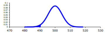.png?revision=1 "hypothesis check data")
Before calculating the probability, it is useful to see how many standard deviations away from the mean the sample mean is. Using the formula for the z-score from chapter 6, you find
\(z=\dfrac{\overline{x}-\mu_{o}}{\sigma / \sqrt{n}}=\dfrac{490-500}{25 / \sqrt{30}}=-2.19\)
This sample mean is more than two standard deviations away from the mean. That seems pretty far, but you should look at the probability too.
On TI-83/84:
\(P(\overline{x}<490 | \mu=500)=\text { normalcdf }(-1 E 99,490,500,25 \div \sqrt{30}) \approx 0.0142\)
\(P(\overline{x}<490 \mu=500)=\text { pnorm }(490,500,25 / \operatorname{sqrt}(30)) \approx 0.0142\)
There is a 1.42% chance that you could find a sample mean less than 490 when the population mean is 500 days. This is really small, so the chances are that the assumption that the population mean is 500 days is wrong, and you can reject the manufacturer’s claim. But how do you quantify really small? Is 5% or 10% or 15% really small? How do you decide?
Before you answer that question, a couple more definitions are needed.
Definition \(\PageIndex{3}\)
Test Statistic : \(z=\dfrac{\overline{x}-\mu_{o}}{\sigma / \sqrt{n}}\) since it is calculated as part of the testing of the hypothesis.
Definition \(\PageIndex{4}\)
p – value : probability that the test statistic will take on more extreme values than the observed test statistic, given that the null hypothesis is true. It is the probability that was calculated above.
Now, how small is small enough? To answer that, you really want to know the types of errors you can make.
There are actually only two errors that can be made. The first error is if you say that \(H_{o}\) is false, when in fact it is true. This means you reject \(H_{o}\) when \(H_{o}\) was true. The second error is if you say that \(H_{o}\) is true, when in fact it is false. This means you fail to reject \(H_{o}\) when \(H_{o}\) is false. The following table organizes this for you:
Type of errors:
| \(H_{o}\) true | \(H_{o}\) false | |
| Reject \(H_{o}\) | Type 1 error | No error |
| Fail to reject \(H_{o}\) | No error | Type II error |
Definition \(\PageIndex{5}\)
Type I Error is rejecting \(H_{o}\) when \(H_{o}\) is true, and
Definition \(\PageIndex{6}\)
Type II Error is failing to reject \(H_{o}\) when \(H_{o}\) is false.
Since these are the errors, then one can define the probabilities attached to each error.
Definition \(\PageIndex{7}\)
\(\alpha\) = P(type I error) = P(rejecting \(H_{o} / H_{o}\) is true)
Definition \(\PageIndex{8}\)
\(\beta\) = P(type II error) = P(failing to reject \(H_{o} / H_{o}\) is false)
\(\alpha\) is also called the level of significance .
Another common concept that is used is Power = \(1-\beta \).
Now there is a relationship between \(\alpha\) and \(\beta\). They are not complements of each other. How are they related?
If \(\alpha\) increases that means the chances of making a type I error will increase. It is more likely that a type I error will occur. It makes sense that you are less likely to make type II errors, only because you will be rejecting \(H_{o}\) more often. You will be failing to reject \(H_{o}\) less, and therefore, the chance of making a type II error will decrease. Thus, as \(\alpha\) increases, \(\beta\) will decrease, and vice versa. That makes them seem like complements, but they aren’t complements. What gives? Consider one more factor – sample size.
Consider if you have a larger sample that is representative of the population, then it makes sense that you have more accuracy then with a smaller sample. Think of it this way, which would you trust more, a sample mean of 490 if you had a sample size of 35 or sample size of 350 (assuming a representative sample)? Of course the 350 because there are more data points and so more accuracy. If you are more accurate, then there is less chance that you will make any error. By increasing the sample size of a representative sample, you decrease both \(\alpha\) and \(\beta\).
Summary of all of this:
- For a certain sample size, n , if \(\alpha\) increases, \(\beta\) decreases.
- For a certain level of significance, \(\alpha\), if n increases, \(\beta\) decreases.
Now how do you find \(\alpha\) and \(\beta\)? Well \(\alpha\) is actually chosen. There are only three values that are usually picked for \(\alpha\): 0.01, 0.05, and 0.10. \(\beta\) is very difficult to find, so usually it isn’t found. If you want to make sure it is small you take as large of a sample as you can afford provided it is a representative sample. This is one use of the Power. You want \(\beta\) to be small and the Power of the test is large. The Power word sounds good.
Which pick of \(\alpha\) do you pick? Well that depends on what you are working on. Remember in this example you are the buyer who is trying to get out of a contract to buy these batteries. If you create a type I error, you said that the batteries are bad when they aren’t, most likely the manufacturer will sue you. You want to avoid this. You might pick \(\alpha\) to be 0.01. This way you have a small chance of making a type I error. Of course this means you have more of a chance of making a type II error. No big deal right? What if the batteries are used in pacemakers and you tell the person that their pacemaker’s batteries are good for 500 days when they actually last less, that might be bad. If you make a type II error, you say that the batteries do last 500 days when they last less, then you have the possibility of killing someone. You certainly do not want to do this. In this case you might want to pick \(\alpha\) as 0.10. If both errors are equally bad, then pick \(\alpha\) as 0.05.
The above discussion is why the choice of \(\alpha\) depends on what you are researching. As the researcher, you are the one that needs to decide what \(\alpha\) level to use based on your analysis of the consequences of making each error is.
If a type I error is really bad, then pick \(\alpha\) = 0.01.
If a type II error is really bad, then pick \(\alpha\) = 0.10
If neither error is bad, or both are equally bad, then pick \(\alpha\) = 0.05
The main thing is to always pick the \(\alpha\) before you collect the data and start the test.
The above discussion was long, but it is really important information. If you don’t know what the errors of the test are about, then there really is no point in making conclusions with the tests. Make sure you understand what the two errors are and what the probabilities are for them.
Now it is time to go back to the example and put this all together. This is the basic structure of testing a hypothesis, usually called a hypothesis test. Since this one has a test statistic involving z, it is also called a z-test. And since there is only one sample, it is usually called a one-sample z-test.
Example \(\PageIndex{2}\) battery example revisited
- State the random variable and the parameter in words.
- State the null and alternative hypothesis and the level of significance.
- A random sample of size n is taken.
- The population standard derivation is known.
- The sample size is at least 30 or the population of the random variable is normally distributed.
- Find the sample statistic, test statistic, and p-value.
- Interpretation
1. x = life of battery
\(\mu\) = mean life of a XJ35 battery
2. \(H_{o} : \mu=500\) days
\(H_{A} : \mu<500\) days
\(\alpha = 0.10\) (from above discussion about consequences)
3. Every hypothesis has some assumptions that be met to make sure that the results of the hypothesis are valid. The assumptions are different for each test. This test has the following assumptions.
- This occurred in this example, since it was stated that a random sample of 30 battery lives were taken.
- This is true, since it was given in the problem.
- The sample size was 30, so this condition is met.
4. The test statistic depends on how many samples there are, what parameter you are testing, and assumptions that need to be checked. In this case, there is one sample and you are testing the mean. The assumptions were checked above.
Sample statistic:
\(\overline{x} = 490\)
Test statistic:
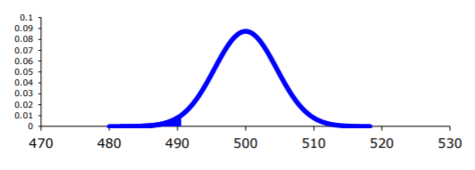.png?revision=1 "hypothesis check data")
Using TI-83/84:
\(P(\overline{x}<490 | \mu=500)=\text { normalcdf }(-1 \mathrm{E} 99,490,500,25 / \sqrt{30}) \approx 0.0142\)
\(P(\overline{x}<490 | \mu=500)=\operatorname{pnorm}(490,500,25 / \operatorname{sqrt}(30)) \approx 0.0142\)
5. Now what? Well, this p-value is 0.0142. This is a lot smaller than the amount of error you would accept in the problem -\(\alpha\) = 0.10. That means that finding a sample mean less than 490 days is unusual to happen if \(H_{o}\) is true. This should make you think that \(H_{o}\) is not true. You should reject \(H_{o}\).
In fact, in general:
Reject \(H_{o}\) if the p-value < \(\alpha\) and
Fail to reject \(H_{o}\) if the p-value \(\geq \alpha\).
6. Since you rejected \(H_{o}\), what does this mean in the real world? That is what goes in the interpretation. Since you rejected the claim by the manufacturer that the mean life of the batteries is 500 days, then you now can believe that your hypothesis was correct. In other words, there is enough evidence to show that the mean life of the battery is less than 500 days.
Now that you know that the batteries last less than 500 days, should you cancel the contract? Statistically, there is evidence that the batteries do not last as long as the manufacturer says they should. However, based on this sample there are only ten days less on average that the batteries last. There may not be practical significance in this case. Ten days do not seem like a large difference. In reality, if the batteries are used in pacemakers, then you would probably tell the patient to have the batteries replaced every year. You have a large buffer whether the batteries last 490 days or 500 days. It seems that it might not be worth it to break the contract over ten days. What if the 10 days was practically significant? Are there any other things you should consider? You might look at the business relationship with the manufacturer. You might also look at how much it would cost to find a new manufacturer. These are also questions to consider before making any changes. What this discussion should show you is that just because a hypothesis has statistical significance does not mean it has practical significance. The hypothesis test is just one part of a research process. There are other pieces that you need to consider.
That’s it. That is what a hypothesis test looks like. All hypothesis tests are done with the same six steps. Those general six steps are outlined below.
- State the random variable and the parameter in words. This is where you are defining what the unknowns are in this problem. x = random variable \(\mu\) = mean of random variable, if the parameter of interest is the mean. There are other parameters you can test, and you would use the appropriate symbol for that parameter.
- State the null and alternative hypotheses and the level of significance \(H_{o} : \mu=\mu_{o}\), where \(\mu_{o}\) is the known mean \(H_{A} : \mu<\mu_{o}\) \(H_{A} : \mu>\mu_{o}\), use the appropriate one for your problem \(H_{A} : \mu \neq \mu_{o}\) Also, state your \(\alpha\) level here.
- State and check the assumptions for a hypothesis test. Each hypothesis test has its own assumptions. They will be stated when the different hypothesis tests are discussed.
- Find the sample statistic, test statistic, and p-value. This depends on what parameter you are working with, how many samples, and the assumptions of the test. The p-value depends on your \(H_{A}\). If you are doing the \(H_{A}\) with the less than, then it is a left-tailed test, and you find the probability of being in that left tail. If you are doing the \(H_{A}\) with the greater than, then it is a right-tailed test, and you find the probability of being in the right tail. If you are doing the \(H_{A}\) with the not equal to, then you are doing a two-tail test, and you find the probability of being in both tails. Because of symmetry, you could find the probability in one tail and double this value to find the probability in both tails.
- Conclusion This is where you write reject \(H_{o}\) or fail to reject \(H_{o}\). The rule is: if the p-value < \(\alpha\), then reject \(H_{o}\). If the p-value \(\geq \alpha\), then fail to reject \(H_{o}\).
- Interpretation This is where you interpret in real world terms the conclusion to the test. The conclusion for a hypothesis test is that you either have enough evidence to show \(H_{A}\) is true, or you do not have enough evidence to show \(H_{A}\) is true.
Sorry, one more concept about the conclusion and interpretation. First, the conclusion is that you reject \(H_{o}\) or you fail to reject \(H_{o}\). Why was it said like this? It is because you never accept the null hypothesis. If you wanted to accept the null hypothesis, then why do the test in the first place? In the interpretation, you either have enough evidence to show \(H_{A}\) is true, or you do not have enough evidence to show \(H_{A}\) is true. You wouldn’t want to go to all this work and then find out you wanted to accept the claim. Why go through the trouble? You always want to show that the alternative hypothesis is true. Sometimes you can do that and sometimes you can’t. It doesn’t mean you proved the null hypothesis; it just means you can’t prove the alternative hypothesis. Here is an example to demonstrate this.
Example \(\PageIndex{3}\) conclusion in hypothesis tests
In the U.S. court system a jury trial could be set up as a hypothesis test. To really help you see how this works, let’s use OJ Simpson as an example. In the court system, a person is presumed innocent until he/she is proven guilty, and this is your null hypothesis. OJ Simpson was a football player in the 1970s. In 1994 his ex-wife and her friend were killed. OJ Simpson was accused of the crime, and in 1995 the case was tried. The prosecutors wanted to prove OJ was guilty of killing his wife and her friend, and that is the alternative hypothesis
\(H_{0}\): OJ is innocent of killing his wife and her friend
\(H_{A}\): OJ is guilty of killing his wife and her friend
In this case, a verdict of not guilty was given. That does not mean that he is innocent of this crime. It means there was not enough evidence to prove he was guilty. Many people believe that OJ was guilty of this crime, but the jury did not feel that the evidence presented was enough to show there was guilt. The verdict in a jury trial is always guilty or not guilty!
The same is true in a hypothesis test. There is either enough or not enough evidence to show that alternative hypothesis. It is not that you proved the null hypothesis true.
When identifying hypothesis, it is important to state your random variable and the appropriate parameter you want to make a decision about. If count something, then the random variable is the number of whatever you counted. The parameter is the proportion of what you counted. If the random variable is something you measured, then the parameter is the mean of what you measured. (Note: there are other parameters you can calculate, and some analysis of those will be presented in later chapters.)
Example \(\PageIndex{4}\) stating hypotheses
Identify the hypotheses necessary to test the following statements:
- The average salary of a teacher is more than $30,000.
- The proportion of students who like math is less than 10%.
- The average age of students in this class differs from 21.
a. x = salary of teacher
\(\mu\) = mean salary of teacher
The guess is that \(\mu>\$ 30,000\) and that is the alternative hypothesis.
The null hypothesis has the same parameter and number with an equal sign.
\(\begin{array}{l}{H_{0} : \mu=\$ 30,000} \\ {H_{A} : \mu>\$ 30,000}\end{array}\)
b. x = number od students who like math
p = proportion of students who like math
The guess is that p < 0.10 and that is the alternative hypothesis.
\(\begin{array}{l}{H_{0} : p=0.10} \\ {H_{A} : p<0.10}\end{array}\)
c. x = age of students in this class
\(\mu\) = mean age of students in this class
The guess is that \(\mu \neq 21\) and that is the alternative hypothesis.
\(\begin{array}{c}{H_{0} : \mu=21} \\ {H_{A} : \mu \neq 21}\end{array}\)
Example \(\PageIndex{5}\) Stating Type I and II Errors and Picking Level of Significance
- The plant-breeding department at a major university developed a new hybrid raspberry plant called YumYum Berry. Based on research data, the claim is made that from the time shoots are planted 90 days on average are required to obtain the first berry with a standard deviation of 9.2 days. A corporation that is interested in marketing the product tests 60 shoots by planting them and recording the number of days before each plant produces its first berry. The sample mean is 92.3 days. The corporation wants to know if the mean number of days is more than the 90 days claimed. State the type I and type II errors in terms of this problem, consequences of each error, and state which level of significance to use.
- A concern was raised in Australia that the percentage of deaths of Aboriginal prisoners was higher than the percent of deaths of non-indigenous prisoners, which is 0.27%. State the type I and type II errors in terms of this problem, consequences of each error, and state which level of significance to use.
a. x = time to first berry for YumYum Berry plant
\(\mu\) = mean time to first berry for YumYum Berry plant
\(\begin{array}{l}{H_{0} : \mu=90} \\ {H_{A} : \mu>90}\end{array}\)
Type I Error: If the corporation does a type I error, then they will say that the plants take longer to produce than 90 days when they don’t. They probably will not want to market the plants if they think they will take longer. They will not market them even though in reality the plants do produce in 90 days. They may have loss of future earnings, but that is all.
Type II error: The corporation do not say that the plants take longer then 90 days to produce when they do take longer. Most likely they will market the plants. The plants will take longer, and so customers might get upset and then the company would get a bad reputation. This would be really bad for the company.
Level of significance: It appears that the corporation would not want to make a type II error. Pick a 10% level of significance, \(\alpha = 0.10\).
b. x = number of Aboriginal prisoners who have died
p = proportion of Aboriginal prisoners who have died
\(\begin{array}{l}{H_{o} : p=0.27 \%} \\ {H_{A} : p>0.27 \%}\end{array}\)
Type I error: Rejecting that the proportion of Aboriginal prisoners who died was 0.27%, when in fact it was 0.27%. This would mean you would say there is a problem when there isn’t one. You could anger the Aboriginal community, and spend time and energy researching something that isn’t a problem.
Type II error: Failing to reject that the proportion of Aboriginal prisoners who died was 0.27%, when in fact it is higher than 0.27%. This would mean that you wouldn’t think there was a problem with Aboriginal prisoners dying when there really is a problem. You risk causing deaths when there could be a way to avoid them.
Level of significance: It appears that both errors may be issues in this case. You wouldn’t want to anger the Aboriginal community when there isn’t an issue, and you wouldn’t want people to die when there may be a way to stop it. It may be best to pick a 5% level of significance, \(\alpha = 0.05\).
Hypothesis testing is really easy if you follow the same recipe every time. The only differences in the various problems are the assumptions of the test and the test statistic you calculate so you can find the p-value. Do the same steps, in the same order, with the same words, every time and these problems become very easy.
Exercise \(\PageIndex{1}\)
For the problems in this section, a question is being asked. This is to help you understand what the hypotheses are. You are not to run any hypothesis tests and come up with any conclusions in this section.
- Eyeglassomatic manufactures eyeglasses for different retailers. They test to see how many defective lenses they made in a given time period and found that 11% of all lenses had defects of some type. Looking at the type of defects, they found in a three-month time period that out of 34,641 defective lenses, 5865 were due to scratches. Are there more defects from scratches than from all other causes? State the random variable, population parameter, and hypotheses.
- According to the February 2008 Federal Trade Commission report on consumer fraud and identity theft, 23% of all complaints in 2007 were for identity theft. In that year, Alaska had 321 complaints of identity theft out of 1,432 consumer complaints ("Consumer fraud and," 2008). Does this data provide enough evidence to show that Alaska had a lower proportion of identity theft than 23%? State the random variable, population parameter, and hypotheses.
- The Kyoto Protocol was signed in 1997, and required countries to start reducing their carbon emissions. The protocol became enforceable in February 2005. In 2004, the mean CO2 emission was 4.87 metric tons per capita. Is there enough evidence to show that the mean CO2 emission is lower in 2010 than in 2004? State the random variable, population parameter, and hypotheses.
- The FDA regulates that fish that is consumed is allowed to contain 1.0 mg/kg of mercury. In Florida, bass fish were collected in 53 different lakes to measure the amount of mercury in the fish. The data for the average amount of mercury in each lake is in Example \(\PageIndex{5}\) ("Multi-disciplinary niser activity," 2013). Do the data provide enough evidence to show that the fish in Florida lakes has more mercury than the allowable amount? State the random variable, population parameter, and hypotheses.
- Eyeglassomatic manufactures eyeglasses for different retailers. They test to see how many defective lenses they made in a given time period and found that 11% of all lenses had defects of some type. Looking at the type of defects, they found in a three-month time period that out of 34,641 defective lenses, 5865 were due to scratches. Are there more defects from scratches than from all other causes? State the type I and type II errors in this case, consequences of each error type for this situation from the perspective of the manufacturer, and the appropriate alpha level to use. State why you picked this alpha level.
- According to the February 2008 Federal Trade Commission report on consumer fraud and identity theft, 23% of all complaints in 2007 were for identity theft. In that year, Alaska had 321 complaints of identity theft out of 1,432 consumer complaints ("Consumer fraud and," 2008). Does this data provide enough evidence to show that Alaska had a lower proportion of identity theft than 23%? State the type I and type II errors in this case, consequences of each error type for this situation from the perspective of the state of Arizona, and the appropriate alpha level to use. State why you picked this alpha level.
- The Kyoto Protocol was signed in 1997, and required countries to start reducing their carbon emissions. The protocol became enforceable in February 2005. In 2004, the mean CO2 emission was 4.87 metric tons per capita. Is there enough evidence to show that the mean CO2 emission is lower in 2010 than in 2004? State the type I and type II errors in this case, consequences of each error type for this situation from the perspective of the agency overseeing the protocol, and the appropriate alpha level to use. State why you picked this alpha level.
- The FDA regulates that fish that is consumed is allowed to contain 1.0 mg/kg of mercury. In Florida, bass fish were collected in 53 different lakes to measure the amount of mercury in the fish. The data for the average amount of mercury in each lake is in Example \(\PageIndex{5}\) ("Multi-disciplinary niser activity," 2013). Do the data provide enough evidence to show that the fish in Florida lakes has more mercury than the allowable amount? State the type I and type II errors in this case, consequences of each error type for this situation from the perspective of the FDA, and the appropriate alpha level to use. State why you picked this alpha level.
1. \(H_{o} : p=0.11, H_{A} : p>0.11\)
3. \(H_{o} : \mu=4.87 \text { metric tons per capita, } H_{A} : \mu<4.87 \text { metric tons per capita }\)
5. See solutions
7. See solutions
IMAGES
COMMENTS
State your research hypothesis as a null hypothesis and alternate hypothesis (H o) and (H a or H 1 ). Collect data in a way designed to test the hypothesis. Perform an appropriate statistical test. Decide whether to reject or fail to reject your null hypothesis.
By understanding its principles, conducting tests properly, and considering real-world applications, you can harness the power of hypothesis testing to unlock valuable insights from your data. Explore the intricacies of hypothesis testing, a cornerstone of statistical analysis.
Hypothesis testing is a method of statistical inference that considers the null hypothesis H ₀ vs. the alternative hypothesis H a, where we are typically looking to assess evidence against H ₀. Such a test is used to compare data sets against one another, or compare a data set against some external standard.
Hypothesis testing is a common statistical tool used in research and data science to support the certainty of findings. The aim of testing is to answer how probable an apparent effect is detected by chance given a random data sample.
Die 1: P(X=x) = 1/6 if x = {1, 2, 3, 4, 5, 6} Die 2: P(X=x) = 1/4 if x = {1, 2} = 1/8 if x = {3, 4, 5, 6} In binary hypothesis testing problems, we’ll often be presented with two choices which we call hypotheses, and we’ll have to decide whether to pick one or the other.
Hypothesis testing in statistics uses sample data to infer the properties of a whole population. These tests determine whether a random sample provides sufficient evidence to conclude an effect or relationship exists in the population.
Article Outline. 1. Introduction to Hypothesis Testing. - Definition and significance in research and data analysis. - Brief historical background. 2. Fundamentals of Hypothesis Testing. -...
In statistics, a hypothesis test calculates some quantity under a given assumption. The result of the test allows us to interpret whether the assumption holds or whether the assumption has been violated. Two concrete examples that we will use a lot in machine learning are: A test that assumes that data has a normal distribution.
Understand what hypothesis testing is and when to use it. Get familiar with various terminologies used in hypothesis testing. Learn the steps of hypothesis testing and how to apply it to various problems. Learn about decision rules and confusion matrix in hypothesis testing.
To understand the process of a hypothesis tests, you need to first have an understanding of what a hypothesis is, which is an educated guess about a parameter. Once you have the hypothesis, you collect data and use the data to make a determination to see if there is enough evidence to show that the hypothesis is true.