how to write null and alternative hypothesis in latex

We love good questions

LaTeX.org on Twitter - follow us

Unanswered topics
Active topics
Impressum and Privacy Policy
About LaTeX
Board index LaTeX General

LaTeX forum ⇒ General ⇒ Null Hyothesis

Null hyothesis.

Post by sbinsaleem » Wed Aug 07, 2013 1:34 pm

Who is online

Users browsing this forum: No registered users and 25 guests

Recommended reading 2024: LaTeXguide.org • LaTeX-Cookbook.net • TikZ.org
News and Articles
Unread posts
Other LaTeX forums
TeXwelt (deutsch)
goLaTeX (deutsch)
TeXnique (français)
Board index
All times are UTC+02:00
Delete all board cookies
Text Formatting
Graphics, Figures & Tables
Math & Science
Fonts & Character Sets
Page Layout
Document Classes
BibTeX, biblatex and biber
MakeIndex, Nomenclature, Glossaries and Acronyms
Conversion Tools
Viewers for PDF, PS, and DVI
Decision Guidance
MiKTeX and proTeXt
TeX Live and MacTeX
Scientific Word/Workplace
Texmaker and TeXstudio
Announcements
Templates, Wizards & Tools
Feature Suggestions
Development
Articles, Essays, and Journal Templates
Theses, Books, Title pages
Presentations and Posters
Curricula Vitae / Résumés
Assignments, Laboratory books and reports
Calendars and Miscellaneous
Community talk
Comments & Wishes
New Members
LaTeX Beginner's Guide

Want to create or adapt books like this? Learn more about how Pressbooks supports open publishing practices.

9.1 Null and Alternative Hypotheses

A hypothesis test is procedure used to determine whether sample data provides enough evidence to determine the validity of claims made about a population.

A hypothesis is a claim or statement about a characteristic of a population of interest to us. A hypothesis test is a way for us to use our sample statistics to test a specific claim [1] about a population parameter.

Null hypothesis is a statement about the value of a population parameter, such as the population mean [latex](\mu)[/latex] or the population proportion [latex](p)[/latex]. It contains the condition of equality and is denoted as H 0 (pronounced H-naught ). The equality condition indicates the status quo, or no change or no effect or no difference . The null hypothesis is assumed true until sample evidence indicates otherwise. Examples: [latex]H_0:\mu = 157[/latex] or [latex]H_0:p = 0.35[/latex]

Alternative hypothesis is the opposite of the null hypothesis. It contains the value of the parameter that we consider plausible and is denoted as H 1 (or H a ). Examples: [latex]H_a:\mu > 157[/latex] or [latex]H_a:p \ne 0.35[/latex]

If a statement contains the condition of equality ([latex]=[/latex] or [latex]\le[/latex] or [latex]\ge[/latex]), then that statement will be expressed as the null hypothesis. Note that [latex]\le[/latex] indicates less than or equal to , while [latex]\ge[/latex] indicates greater than or equal to . In both cases, the equal to (the condition of equality) part is present.

Understanding the Language of Hypothesis Testing

A climatologist wants to check the claim on a Wikipedia article that San Diego averages a maximum of 66 days of measurable precipitation per year.

Since the question states that “ San Diego averages a maximum of 66 days … “, the parameter of interest is the average (or the mean).

Note that for this class we’ll use the words mean and average interchangeably, although mathematically they can be different. Read more about Mean vs Average.

The actual average days of annual precipitation for San Diego is not something the climatologist knows otherwise they could easily see if that average is no more than 66 days. Therefore the unknown parameter here for the researcher is the average number of days of measurable precipitation per year in San Diego. Let’s call that average [latex]\mu[/latex].

Let [latex]\mu =[/latex] average days of measurable precipitation per year in San Diego

Let’s write the claim using mathematical symbols:

the average days of measurable precipitation per year in San Diego [latex]= \mu[/latex]

is no more than 66 [latex]\rightarrow[/latex] [latex]\le 66[/latex]

Putting it together, the claim is: [latex]\mu\le 66[/latex]. This claim contains the condition of equality. The opposite of this claim is [latex]\mu > 66[/latex].

Of the two statements above, the null hypothesis, [latex]H_o[/latex], is the one that has the [latex]=[/latex] sign while other statement is the alternative hypothesis, [latex]H_a \ ([/latex]or [latex]H_1)[/latex]. We can write:

\[H_o: \mu \le 66\]\[H_a: \mu > 66\]

We can represent the null and the alternative hypotheses on a number line. Since the null hypothesis is [latex]\mu\le 66[/latex], the part of the number line representing this inequality is shown by the blue arrow below. This is the side that favors the null. The other unshaded side on the number line represents the alternative hypothesis, which in this case is [latex]\mu > 66[/latex].

Some textbook authors prefer to write the null hypothesis for this example as [latex]H_o:\mu=66[/latex], where 66 is the highest value on the null side. When testing the alternative against the null, if we can reasonably be assured that the unknown parameter is greater than 66, then it’s automatically greater than any value less than 66. With this approach, we write the null and the alternative as follows:

\[H_o: \mu = 66\]\[H_a: \mu > 66\]

An economist claims that lower than 81% of investment portfolios went up in value this past year.

Since the 81% given is the percentage of investment portfolios that went up in value this past year, that 81% represents the proportion of portfolios that increased their value. The economist believes that the percentage of portfolios that increased their value is lower, but they don’t know that actual percentage. The unknown parameter here is the proportion (the decimal equivalent of the percentage) of investment portfolios that went up in value. Let’s call that proportion p .

Let [latex]p =[/latex] proportion of investment portfolios that went up in value this past year

The economist believes that this actual proportion is lower than 81% or 0.81. In symbols:

[latex]p<0.81[/latex]

This is an example of a claim that doesn’t contain the condition of equality. The opposite of the claim is:

[latex]p\ge0.81[/latex]

[latex]H_0: p \ge 0.81[/latex][latex]H_a: p

[latex]H_0: p = 0.81[/latex][latex]H_a: p

The mean price of mid-sized cars in a region is 42400. A test is conducted to see if the claim is true.

Since the test is to see if the claim that the mean price of 42400 is true for mid-sized cars, this would be a test for the mean . The unknown parameter here is the mean price of all mid-sized cars. Let’s call that average [latex]\mu[/latex].

Let [latex]\mu =[/latex] mean price of mid-sized cars in a region

We’d like to see if this mean, [latex]\mu[/latex], is equal to 42400. Let’s write the claim about the mean using mathematical symbols:

[latex]\mu = 42400[/latex]

This is an example of a claim that contains condition of equality. The opposite of this claim is [latex]\mu \ne 42400[/latex].

\[H_o: \mu = 42400\]\[H_a: \mu \ne 42400\]

ADDITIONAL Practice

Test statistic is the z or t-score of the sample data. Some textbooks define test statistic as the sample statistic (mean, proportion, difference of means, etc.) and the z or t-score associated with that sample statistic as the standardized test statistic .

Tail-type of a test is the direction favored by the alternative hypothesis.

Types of Tail

Review Types of Tests .

For a visual explanation, watch the following video:

How do you decide the tail type for your study? Choosing between One-tailed or a two-tailed test for your data analysis

Lumen Learning ↵

Share This Book

Show All Code
Hide All Code

Latex for hypothesis testing

Jeffrey liang.

R Code can be found in here

Distribution

\[ P(\mathcal{X}=k)\ = {n \choose k}p^k(1-p)^{n-k} \]

Normal Distribution

$P(\mathcal{X}=k)\ = \frac{1}{\sqrt{2\pi}\sigma}*e^{-\frac{(x-\mu)^2}{2\sigma^2}}$

One Group t-test

Left tailed.

$H_0$ : there’s no difference betwee sample mean and the true mean

$H_1$ : the sample mean is lower than the true mean

$\bar{x} = \frac{\sum_{i=1}^n{x_i}}{n}$

$s_d = \sqrt{\sum_{i=1}^n{(x_i - \bar{x})^2}/(n-1)}$

$t = \frac{\bar{x} - 0}{s_d/\sqrt{n}}$

$Reject ~ H_0 ~ if ~ t<t_{n-1,\alpha}$

$Fail ~ reject ~ H_0 ~ if ~ t>t_{n-1,\alpha}$

$CI : (-\infty,\bar{x} - t_{df,\alpha}*sd/\sqrt{n})$

right tailed

$H_1$ : the sample mean is greater than the true mean

$Reject ~ H_0 ~ if ~ t>t_{n-1,1-\alpha}$

$Fail ~ reject ~ H_0 ~ if ~ t<t_{n-1,1-\alpha}$

$CI : (\bar{x} + t_{df,1-\alpha}*sd/\sqrt{n},\infty)$

$H_1$ : the sample mean is different from the true mean

$Reject ~ H_0 ~ if ~ |t|<t_{n-1,1-\alpha/2}$

$Fail ~ reject ~ H_0 ~ if ~ |t|<t_{n-1,1 - \alpha/2}$

$CI : (\bar{x} - t_{df,1-\alpha/2}*sd/\sqrt{n} ,\bar{x} + t_{df,1-\alpha/2}*sd/\sqrt{n})$

$H_0$ : there’s no difference betwee difference

$H_1$ : the difference is different

$\bar{d} = \frac{\sum_{i=1}^n{d_i}}{n}$

$s_d = \sqrt{\sum_{i=1}^n{(d_i - \bar{d})^2}/(n-1)}$

$t = \frac{\bar{d} - 0}{s_d/\sqrt{n}}$

$CI : (\bar{d} - t_{df,1-\alpha/2}*sd/\sqrt{n} ,\bar{d} + t_{df,1-\alpha/2}*sd/\sqrt{n})$

Two Group testing

Variance test.

$H_0$ : the variances between group are equal(no difference)

$H_1$ : the variances between group are not equal(there’s difference)

$s_{x_1} = \sqrt{\sum_{i=1}^{n_1}(x_i - \bar{x_1})^2/(n_1-1)}$

$s_{x_2} = \sqrt{\sum_{j=1}^{n_2}(x_i - \bar{x_2})^2/(n_2-1)}$

$F = s_1^2/s_2^2 \sim F_{n_1-1,n_2-1}$

$Reject ~ H_0 ~ if ~ F>F_{n_1-1,n_2-1,1-\alpha/2} ~ OR ~ F<F_{n_1-1,n_2-1,\alpha/2}$

$Fail ~ reject ~ H_0 ~ if ~ F_{n_1-1,n_2-1,\alpha/2}<F<F_{n_1-1,n_2-1,1-\alpha/2}$

t-test with equal variance

$H_0$ : the means between group are equal(no difference)

$H_1$ : the means between group are not equal(there’s difference)

$s_{pool} = \frac{(n_1-1)s_1 + (n_2 -1)s_2}{n_1+n_2-2}$

$t = \frac{\bar{X_1} - \bar{X_2}}{s_{pool}\times\sqrt{\frac{1}{n_1}+\frac{1}{n_2}}}$

$Reject ~ H_0 ~ if ~ |t|>t_{df,1-\alpha/2}$

$Fail ~ reject ~ H_0 ~ if ~ |t|<t_{df,1-\alpha/2}$

$CI = (\bar{X_1}-\bar{X_2} ~ - ~ t_{df,1-\alpha/2}s_{pool}/\sqrt{1/n_1+1/n_2},\bar{X_1}-\bar{X_2} ~ + ~ t_{df,1-\alpha/2}s_{pool}/\sqrt{1/n_1+1/n_2} )$

t-test with unequal variance

$\bar{X_1} - \bar{X_2} \sim N(\mu_1-\mu_2,\frac{\sigma_1^2}{n_1}+\frac{\sigma_2^2}{n_2})$ if we know the population variance

$t = \frac{\bar{X_1} - \bar{X_2}}{\sqrt{\frac{s_1^2}{n_1}+\frac{s_2^2}{n_2}}}~\sim t_{d''}$

$d' = round(d'') = \frac{(\frac{s_1^2}{n_1}+\frac{s_2^2}{n_2})^2}{\frac{s_1^2}{n_1}^2/(n_1-1)+\frac{s_2^2}{n_2}^2/(n_2-1)}$

$CI = (\bar{X_1}-\bar{X_2} ~ - ~ t_{df,1-\alpha/2}\sqrt{\frac{s_1^2}{n_1}+\frac{s_2^2}{n_2}},\bar{X_1}-\bar{X_2} ~ + ~ t_{df,1-\alpha/2}\sqrt{\frac{s_1^2}{n_1}+\frac{s_2^2}{n_2}})$

Multigroup Camparison

$H_0$ : there’s no difference between groups

$H_1$ : at least one group is different from the other groups

$Between~Sum~of~Square = \sum_{i=1}^k\sum_{j=1}^{n_i}(\bar{y_i} - \bar{\bar{y}})^2=\sum_i^kn_i\bar{y_i}^2-\frac{y_{..}^2}{n}$

$Within~Sum~of~Square = \sum_{i=1}^k\sum_{j=1}^{n_i}(y_{ij}-\bar{y_i})^2=\sum_i^k(n_i-1)s_i^2$

$Between~Mean~Square = \frac{\sum_{i=1}^k\sum_{j=1}^{n_i}(\bar{y_i} - \bar{\bar{y}})^2}{k-1}$

$Within~Mean~Square = \frac{\sum_{i=1}^k\sum_{j=1}^{n_i}(y_{ij}-\bar{y_i})^2}{n-k}$

$F_{statistics} = \frac{Between~Mean~Square}{Within~Mean~Square} \sim F(k-1,n-k)$

$Reject ~ H_0 ~ if ~ F>F_{k-1,n-k,1-\alpha}$

$Fail ~ reject ~ H_0 ~ if ~F<F_{k-1,n-k,1-\alpha}$

Proportion testing

Normal approximation, homogeneity chi-sq test.

$H_0 :p_{1j} =p_{2j}=...=p_{ij}$ the proportion among $group_i$ are equal …

$H_1$ : For at least one column there’re two row i and i’ where the proability are not the same.

$\mathcal{X}^2 = \sum_i^{row}\sum_j^{col}\frac{(n_{ij}-E_{ij})^2}{E_{ij}} \sim \mathcal{X}^2_{df = (row-1)\times(col-1)}$

$Reject ~ H_0 ~ if ~ \mathcal{X}^2>\mathcal{X}^2_{(r-1))*(c-1),1-\alpha}$

$Fail ~ reject ~ H_0 ~ if ~\mathcal{X}^2<\mathcal{X}^2_{(r-1))*(c-1),1-\alpha}$

Independent test

$H_0$ : Group A and Group B are independet

$H_1$ : Group A and Group B are dependet/associate

Fisher Exact

Mcnemar test.

9.1 Null and Alternative Hypotheses

The actual test begins by considering two hypotheses . They are called the null hypothesis and the alternative hypothesis . These hypotheses contain opposing viewpoints.

H 0 , the — null hypothesis: a statement of no difference between sample means or proportions or no difference between a sample mean or proportion and a population mean or proportion. In other words, the difference equals 0.

H a —, the alternative hypothesis: a claim about the population that is contradictory to H 0 and what we conclude when we reject H 0 .

Since the null and alternative hypotheses are contradictory, you must examine evidence to decide if you have enough evidence to reject the null hypothesis or not. The evidence is in the form of sample data.

After you have determined which hypothesis the sample supports, you make a decision. There are two options for a decision. They are reject H 0 if the sample information favors the alternative hypothesis or do not reject H 0 or decline to reject H 0 if the sample information is insufficient to reject the null hypothesis.

Mathematical Symbols Used in H 0 and H a :


equal (=)	not equal (≠) greater than (>) less than (<)
greater than or equal to (≥)	less than (<)
less than or equal to (≤)	more than (>)

H 0 always has a symbol with an equal in it. H a never has a symbol with an equal in it. The choice of symbol depends on the wording of the hypothesis test. However, be aware that many researchers use = in the null hypothesis, even with > or < as the symbol in the alternative hypothesis. This practice is acceptable because we only make the decision to reject or not reject the null hypothesis.

Example 9.1

H 0 : No more than 30 percent of the registered voters in Santa Clara County voted in the primary election. p ≤ 30 H a : More than 30 percent of the registered voters in Santa Clara County voted in the primary election. p > 30

A medical trial is conducted to test whether or not a new medicine reduces cholesterol by 25 percent. State the null and alternative hypotheses.

Example 9.2

We want to test whether the mean GPA of students in American colleges is different from 2.0 (out of 4.0). The null and alternative hypotheses are the following: H 0 : μ = 2.0 H a : μ ≠ 2.0

We want to test whether the mean height of eighth graders is 66 inches. State the null and alternative hypotheses. Fill in the correct symbol (=, ≠, ≥, <, ≤, >) for the null and alternative hypotheses.

H 0 : μ __ 66
H a : μ __ 66

Example 9.3

We want to test if college students take fewer than five years to graduate from college, on the average. The null and alternative hypotheses are the following: H 0 : μ ≥ 5 H a : μ < 5

We want to test if it takes fewer than 45 minutes to teach a lesson plan. State the null and alternative hypotheses. Fill in the correct symbol ( =, ≠, ≥, <, ≤, >) for the null and alternative hypotheses.

H 0 : μ __ 45
H a : μ __ 45

Example 9.4

An article on school standards stated that about half of all students in France, Germany, and Israel take advanced placement exams and a third of the students pass. The same article stated that 6.6 percent of U.S. students take advanced placement exams and 4.4 percent pass. Test if the percentage of U.S. students who take advanced placement exams is more than 6.6 percent. State the null and alternative hypotheses. H 0 : p ≤ 0.066 H a : p > 0.066

On a state driver’s test, about 40 percent pass the test on the first try. We want to test if more than 40 percent pass on the first try. Fill in the correct symbol (=, ≠, ≥, <, ≤, >) for the null and alternative hypotheses.

H 0 : p __ 0.40
H a : p __ 0.40

Collaborative Exercise

Bring to class a newspaper, some news magazines, and some internet articles. In groups, find articles from which your group can write null and alternative hypotheses. Discuss your hypotheses with the rest of the class.

This book may not be used in the training of large language models or otherwise be ingested into large language models or generative AI offerings without OpenStax's permission.

Want to cite, share, or modify this book? This book uses the Creative Commons Attribution License and you must attribute Texas Education Agency (TEA). The original material is available at: https://www.texasgateway.org/book/tea-statistics . Changes were made to the original material, including updates to art, structure, and other content updates.

Access for free at https://openstax.org/books/statistics/pages/1-introduction

Authors: Barbara Illowsky, Susan Dean
Publisher/website: OpenStax
Book title: Statistics
Publication date: Mar 27, 2020
Location: Houston, Texas
Book URL: https://openstax.org/books/statistics/pages/1-introduction
Section URL: https://openstax.org/books/statistics/pages/9-1-null-and-alternative-hypotheses

© Apr 16, 2024 Texas Education Agency (TEA). The OpenStax name, OpenStax logo, OpenStax book covers, OpenStax CNX name, and OpenStax CNX logo are not subject to the Creative Commons license and may not be reproduced without the prior and express written consent of Rice University.

Have a language expert improve your writing

Run a free plagiarism check in 10 minutes, generate accurate citations for free.

Knowledge Base
Null and Alternative Hypotheses | Definitions & Examples

Null & Alternative Hypotheses | Definitions, Templates & Examples

Published on May 6, 2022 by Shaun Turney . Revised on June 22, 2023.

The null and alternative hypotheses are two competing claims that researchers weigh evidence for and against using a statistical test :

Null hypothesis ( H 0 ): There’s no effect in the population .
Alternative hypothesis ( H a or H 1 ) : There’s an effect in the population.

Answering your research question with hypotheses, what is a null hypothesis, what is an alternative hypothesis, similarities and differences between null and alternative hypotheses, how to write null and alternative hypotheses, other interesting articles, frequently asked questions.

The null and alternative hypotheses offer competing answers to your research question . When the research question asks “Does the independent variable affect the dependent variable?”:

The null hypothesis ( H 0 ) answers “No, there’s no effect in the population.”
The alternative hypothesis ( H a ) answers “Yes, there is an effect in the population.”

The null and alternative are always claims about the population. That’s because the goal of hypothesis testing is to make inferences about a population based on a sample . Often, we infer whether there’s an effect in the population by looking at differences between groups or relationships between variables in the sample. It’s critical for your research to write strong hypotheses .

You can use a statistical test to decide whether the evidence favors the null or alternative hypothesis. Each type of statistical test comes with a specific way of phrasing the null and alternative hypothesis. However, the hypotheses can also be phrased in a general way that applies to any test.

Here's why students love Scribbr's proofreading services

Discover proofreading & editing

The null hypothesis is the claim that there’s no effect in the population.

If the sample provides enough evidence against the claim that there’s no effect in the population ( p ≤ α), then we can reject the null hypothesis . Otherwise, we fail to reject the null hypothesis.

Although “fail to reject” may sound awkward, it’s the only wording that statisticians accept . Be careful not to say you “prove” or “accept” the null hypothesis.

Null hypotheses often include phrases such as “no effect,” “no difference,” or “no relationship.” When written in mathematical terms, they always include an equality (usually =, but sometimes ≥ or ≤).

You can never know with complete certainty whether there is an effect in the population. Some percentage of the time, your inference about the population will be incorrect. When you incorrectly reject the null hypothesis, it’s called a type I error . When you incorrectly fail to reject it, it’s a type II error.

Examples of null hypotheses

The table below gives examples of research questions and null hypotheses. There’s always more than one way to answer a research question, but these null hypotheses can help you get started.

	( )

Does tooth flossing affect the number of cavities?	Tooth flossing has on the number of cavities.	test: The mean number of cavities per person does not differ between the flossing group (µ ) and the non-flossing group (µ ) in the population; µ = µ .
Does the amount of text highlighted in the textbook affect exam scores?	The amount of text highlighted in the textbook has on exam scores.	: There is no relationship between the amount of text highlighted and exam scores in the population; β = 0.
Does daily meditation decrease the incidence of depression?	Daily meditation the incidence of depression.*	test: The proportion of people with depression in the daily-meditation group ( ) is greater than or equal to the no-meditation group ( ) in the population; ≥ .

*Note that some researchers prefer to always write the null hypothesis in terms of “no effect” and “=”. It would be fine to say that daily meditation has no effect on the incidence of depression and p 1 = p 2 .

The alternative hypothesis ( H a ) is the other answer to your research question . It claims that there’s an effect in the population.

Often, your alternative hypothesis is the same as your research hypothesis. In other words, it’s the claim that you expect or hope will be true.

The alternative hypothesis is the complement to the null hypothesis. Null and alternative hypotheses are exhaustive, meaning that together they cover every possible outcome. They are also mutually exclusive, meaning that only one can be true at a time.

Alternative hypotheses often include phrases such as “an effect,” “a difference,” or “a relationship.” When alternative hypotheses are written in mathematical terms, they always include an inequality (usually ≠, but sometimes < or >). As with null hypotheses, there are many acceptable ways to phrase an alternative hypothesis.

Examples of alternative hypotheses

The table below gives examples of research questions and alternative hypotheses to help you get started with formulating your own.



Does tooth flossing affect the number of cavities?	Tooth flossing has an on the number of cavities.	test: The mean number of cavities per person differs between the flossing group (µ ) and the non-flossing group (µ ) in the population; µ ≠ µ .
Does the amount of text highlighted in a textbook affect exam scores?	The amount of text highlighted in the textbook has an on exam scores.	: There is a relationship between the amount of text highlighted and exam scores in the population; β ≠ 0.
Does daily meditation decrease the incidence of depression?	Daily meditation the incidence of depression.	test: The proportion of people with depression in the daily-meditation group ( ) is less than the no-meditation group ( ) in the population; < .

Null and alternative hypotheses are similar in some ways:

They’re both answers to the research question.
They both make claims about the population.
They’re both evaluated by statistical tests.

However, there are important differences between the two types of hypotheses, summarized in the following table.


	A claim that there is in the population.	A claim that there is in the population.


	Equality symbol (=, ≥, or ≤)	Inequality symbol (≠, <, or >)
	Rejected	Supported
	Failed to reject	Not supported

Prevent plagiarism. Run a free check.

To help you write your hypotheses, you can use the template sentences below. If you know which statistical test you’re going to use, you can use the test-specific template sentences. Otherwise, you can use the general template sentences.

General template sentences

The only thing you need to know to use these general template sentences are your dependent and independent variables. To write your research question, null hypothesis, and alternative hypothesis, fill in the following sentences with your variables:

Does independent variable affect dependent variable ?

Null hypothesis ( H 0 ): Independent variable does not affect dependent variable.
Alternative hypothesis ( H a ): Independent variable affects dependent variable.

Test-specific template sentences

Once you know the statistical test you’ll be using, you can write your hypotheses in a more precise and mathematical way specific to the test you chose. The table below provides template sentences for common statistical tests.

	( )
test with two groups	The mean dependent variable does not differ between group 1 (µ ) and group 2 (µ ) in the population; µ = µ .	The mean dependent variable differs between group 1 (µ ) and group 2 (µ ) in the population; µ ≠ µ .
with three groups	The mean dependent variable does not differ between group 1 (µ ), group 2 (µ ), and group 3 (µ ) in the population; µ = µ = µ .	The mean dependent variable of group 1 (µ ), group 2 (µ ), and group 3 (µ ) are not all equal in the population.
	There is no correlation between independent variable and dependent variable in the population; ρ = 0.	There is a correlation between independent variable and dependent variable in the population; ρ ≠ 0.
	There is no relationship between independent variable and dependent variable in the population; β = 0.	There is a relationship between independent variable and dependent variable in the population; β ≠ 0.
Two-proportions test	The dependent variable expressed as a proportion does not differ between group 1 ( ) and group 2 ( ) in the population; = .	The dependent variable expressed as a proportion differs between group 1 ( ) and group 2 ( ) in the population; ≠ .

Note: The template sentences above assume that you’re performing one-tailed tests . One-tailed tests are appropriate for most studies.

If you want to know more about statistics , methodology , or research bias , make sure to check out some of our other articles with explanations and examples.

Normal distribution
Descriptive statistics
Measures of central tendency
Correlation coefficient

Methodology

Cluster sampling
Stratified sampling
Types of interviews
Cohort study
Thematic analysis

Research bias

Implicit bias
Cognitive bias
Survivorship bias
Availability heuristic
Nonresponse bias
Regression to the mean

Hypothesis testing is a formal procedure for investigating our ideas about the world using statistics. It is used by scientists to test specific predictions, called hypotheses , by calculating how likely it is that a pattern or relationship between variables could have arisen by chance.

Null and alternative hypotheses are used in statistical hypothesis testing . The null hypothesis of a test always predicts no effect or no relationship between variables, while the alternative hypothesis states your research prediction of an effect or relationship.

The null hypothesis is often abbreviated as H 0 . When the null hypothesis is written using mathematical symbols, it always includes an equality symbol (usually =, but sometimes ≥ or ≤).

The alternative hypothesis is often abbreviated as H a or H 1 . When the alternative hypothesis is written using mathematical symbols, it always includes an inequality symbol (usually ≠, but sometimes < or >).

A research hypothesis is your proposed answer to your research question. The research hypothesis usually includes an explanation (“ x affects y because …”).

A statistical hypothesis, on the other hand, is a mathematical statement about a population parameter. Statistical hypotheses always come in pairs: the null and alternative hypotheses . In a well-designed study , the statistical hypotheses correspond logically to the research hypothesis.

Cite this Scribbr article

If you want to cite this source, you can copy and paste the citation or click the “Cite this Scribbr article” button to automatically add the citation to our free Citation Generator.

Turney, S. (2023, June 22). Null & Alternative Hypotheses | Definitions, Templates & Examples. Scribbr. Retrieved August 21, 2024, from https://www.scribbr.com/statistics/null-and-alternative-hypotheses/

Is this article helpful?

Shaun Turney

Other students also liked, inferential statistics | an easy introduction & examples, hypothesis testing | a step-by-step guide with easy examples, type i & type ii errors | differences, examples, visualizations, what is your plagiarism score.

Want to create or adapt books like this? Learn more about how Pressbooks supports open publishing practices.

Hypothesis Testing with One Sample

Null and Alternative Hypotheses

OpenStaxCollege

[latexpage]

The actual test begins by considering two hypotheses . They are called the null hypothesis and the alternative hypothesis . These hypotheses contain opposing viewpoints.

H 0 : The null hypothesis: It is a statement about the population that either is believed to be true or is used to put forth an argument unless it can be shown to be incorrect beyond a reasonable doubt.

H a : The alternative hypothesis: It is a claim about the population that is contradictory to H 0 and what we conclude when we reject H 0 .

After you have determined which hypothesis the sample supports, you make a decision. There are two options for a decision. They are “reject H 0 ” if the sample information favors the alternative hypothesis or “do not reject H 0 ” or “decline to reject H 0 ” if the sample information is insufficient to reject the null hypothesis.

Mathematical Symbols Used in H 0 and H a :


equal (=)	not equal (≠) greater than (>) less than (<)
greater than or equal to (≥)	less than (<)
less than or equal to (≤)	more than (>)

H 0 always has a symbol with an equal in it. H a never has a symbol with an equal in it. The choice of symbol depends on the wording of the hypothesis test. However, be aware that many researchers (including one of the co-authors in research work) use = in the null hypothesis, even with > or < as the symbol in the alternative hypothesis. This practice is acceptable because we only make the decision to reject or not reject the null hypothesis.

H 0 : No more than 30% of the registered voters in Santa Clara County voted in the primary election. p ≤ 30

A medical trial is conducted to test whether or not a new medicine reduces cholesterol by 25%. State the null and alternative hypotheses.

H 0 : The drug reduces cholesterol by 25%. p = 0.25

H a : The drug does not reduce cholesterol by 25%. p ≠ 0.25

We want to test whether the mean GPA of students in American colleges is different from 2.0 (out of 4.0). The null and alternative hypotheses are:

H 0 : μ = 2.0

H 0 : μ = 66
H a : μ ≠ 66

We want to test if college students take less than five years to graduate from college, on the average. The null and alternative hypotheses are:

H 0 : μ ≥ 5

H 0 : μ ≥ 45
H a : μ < 45

In an issue of U. S. News and World Report , an article on school standards stated that about half of all students in France, Germany, and Israel take advanced placement exams and a third pass. The same article stated that 6.6% of U.S. students take advanced placement exams and 4.4% pass. Test if the percentage of U.S. students who take advanced placement exams is more than 6.6%. State the null and alternative hypotheses.

H 0 : p ≤ 0.066

On a state driver’s test, about 40% pass the test on the first try. We want to test if more than 40% pass on the first try. Fill in the correct symbol (=, ≠, ≥, <, ≤, >) for the null and alternative hypotheses.

H 0 : p = 0.40
H a : p > 0.40

<!– ??? –>

Bring to class a newspaper, some news magazines, and some Internet articles . In groups, find articles from which your group can write null and alternative hypotheses. Discuss your hypotheses with the rest of the class.

Chapter Review

In a hypothesis test , sample data is evaluated in order to arrive at a decision about some type of claim. If certain conditions about the sample are satisfied, then the claim can be evaluated for a population. In a hypothesis test, we:

Formula Review

H 0 and H a are contradictory.

has:	equal (=)	greater than or equal to (≥)	less than or equal to (≤)
has:	not equal (≠) greater than (>) less than (<)	less than (<)	greater than (>)

If α ≤ p -value, then do not reject H 0 .

If α > p -value, then reject H 0 .

α is preconceived. Its value is set before the hypothesis test starts. The p -value is calculated from the data.

You are testing that the mean speed of your cable Internet connection is more than three Megabits per second. What is the random variable? Describe in words.

The random variable is the mean Internet speed in Megabits per second.

You are testing that the mean speed of your cable Internet connection is more than three Megabits per second. State the null and alternative hypotheses.

The American family has an average of two children. What is the random variable? Describe in words.

The random variable is the mean number of children an American family has.

The mean entry level salary of an employee at a company is 💲58,000. You believe it is higher for IT professionals in the company. State the null and alternative hypotheses.

A sociologist claims the probability that a person picked at random in Times Square in New York City is visiting the area is 0.83. You want to test to see if the proportion is actually less. What is the random variable? Describe in words.

The random variable is the proportion of people picked at random in Times Square visiting the city.

A sociologist claims the probability that a person picked at random in Times Square in New York City is visiting the area is 0.83. You want to test to see if the claim is correct. State the null and alternative hypotheses.

In a population of fish, approximately 42% are female. A test is conducted to see if, in fact, the proportion is less. State the null and alternative hypotheses.

Suppose that a recent article stated that the mean time spent in jail by a first–time convicted burglar is 2.5 years. A study was then done to see if the mean time has increased in the new century. A random sample of 26 first-time convicted burglars in a recent year was picked. The mean length of time in jail from the survey was 3 years with a standard deviation of 1.8 years. Suppose that it is somehow known that the population standard deviation is 1.5. If you were conducting a hypothesis test to determine if the mean length of jail time has increased, what would the null and alternative hypotheses be? The distribution of the population is normal.

A random survey of 75 death row inmates revealed that the mean length of time on death row is 17.4 years with a standard deviation of 6.3 years. If you were conducting a hypothesis test to determine if the population mean time on death row could likely be 15 years, what would the null and alternative hypotheses be?

H 0 : __________
H a : __________
H 0 : μ = 15
H a : μ ≠ 15

The National Institute of Mental Health published an article stating that in any one-year period, approximately 9.5 percent of American adults suffer from depression or a depressive illness. Suppose that in a survey of 100 people in a certain town, seven of them suffered from depression or a depressive illness. If you were conducting a hypothesis test to determine if the true proportion of people in that town suffering from depression or a depressive illness is lower than the percent in the general adult American population, what would the null and alternative hypotheses be?

Some of the following statements refer to the null hypothesis, some to the alternate hypothesis.

State the null hypothesis, H 0 , and the alternative hypothesis. H a , in terms of the appropriate parameter ( μ or p ).

The mean number of years Americans work before retiring is 34.
At most 60% of Americans vote in presidential elections.
The mean starting salary for San Jose State University graduates is at least 💲100,000 per year.
Twenty-nine percent of high school seniors get drunk each month.
Fewer than 5% of adults ride the bus to work in Los Angeles.
The mean number of cars a person owns in her lifetime is not more than ten.
About half of Americans prefer to live away from cities, given the choice.
Europeans have a mean paid vacation each year of six weeks.
The chance of developing breast cancer is under 11% for women.
Private universities’ mean tuition cost is more than 💲20,000 per year.
H 0 : μ = 34; H a : μ ≠ 34
H 0 : p ≤ 0.60; H a : p > 0.60
H 0 : μ ≥ 100,000; H a : μ < 100,000
H 0 : p = 0.29; H a : p ≠ 0.29
H 0 : p = 0.05; H a : p < 0.05
H 0 : μ ≤ 10; H a : μ > 10
H 0 : p = 0.50; H a : p ≠ 0.50
H 0 : μ = 6; H a : μ ≠ 6
H 0 : p ≥ 0.11; H a : p < 0.11
H 0 : μ ≤ 20,000; H a : μ > 20,000

Over the past few decades, public health officials have examined the link between weight concerns and teen girls’ smoking. Researchers surveyed a group of 273 randomly selected teen girls living in Massachusetts (between 12 and 15 years old). After four years the girls were surveyed again. Sixty-three said they smoked to stay thin. Is there good evidence that more than thirty percent of the teen girls smoke to stay thin? The alternative hypothesis is:

p < 0.30
p > 0.30

A statistics instructor believes that fewer than 20% of Evergreen Valley College (EVC) students attended the opening night midnight showing of the latest Harry Potter movie. She surveys 84 of her students and finds that 11 attended the midnight showing. An appropriate alternative hypothesis is:

p > 0.20
p < 0.20

Previously, an organization reported that teenagers spent 4.5 hours per week, on average, on the phone. The organization thinks that, currently, the mean is higher. Fifteen randomly chosen teenagers were asked how many hours per week they spend on the phone. The sample mean was 4.75 hours with a sample standard deviation of 2.0. Conduct a hypothesis test. The null and alternative hypotheses are:

H o : $\overline{x}$ = 4.5, H a : $\overline{x}$ > 4.5
H o : μ ≥ 4.5, H a : μ < 4.5
H o : μ = 4.75, H a : μ > 4.75
H o : μ = 4.5, H a : μ > 4.5

Data from the National Institute of Mental Health. Available online at http://www.nimh.nih.gov/publicat/depression.cfm.

Knowledge Base
Annotating with Hypothesis

Formatting Annotations with LaTeX

The Hypothesis editor supports LaTeX formatting markup, allowing the use of advanced math and scientific typography within annotations.

Also see our articles on adding links and images , embedding videos , and using Markdown .

If you’re wondering what LaTeX is or what it’s used for, here’s a pretty good primer .

We use the KaTeX library to render LaTeX. Here is a full list of supported functions and notation .

To use LaTeX formatting in Hypothesis, simply begin and end the markup with two dollar-signs ( $$ ). For example: $$\sum_{\mathclap{1\le i\le n}} x_{i}$$

You can also use the editor toolbar:

Location of LaTeX button and where to insert LaTeX code

Exporting and Importing Annotations
Keyboard Shortcuts for Hypothesis
Using Hypothesis with JSTOR
A Hypothesis-Compatible Way to Use Adobe Acrobat to Split a PDF
Hypothesis and Screen Readers
Citing Hypothesis Annotations

Ask a Question

Have a thesis expert improve your writing

Check your thesis for plagiarism in 10 minutes, generate your apa citations for free.

Knowledge Base
Null and Alternative Hypotheses | Definitions & Examples

Null and Alternative Hypotheses | Definitions & Examples

Published on 5 October 2022 by Shaun Turney . Revised on 6 December 2022.

The null and alternative hypotheses are two competing claims that researchers weigh evidence for and against using a statistical test :

Null hypothesis (H 0 ): There’s no effect in the population .
Alternative hypothesis (H A ): There’s an effect in the population.

The effect is usually the effect of the independent variable on the dependent variable .

Answering your research question with hypotheses, what is a null hypothesis, what is an alternative hypothesis, differences between null and alternative hypotheses, how to write null and alternative hypotheses, frequently asked questions about null and alternative hypotheses.

The null and alternative hypotheses offer competing answers to your research question . When the research question asks “Does the independent variable affect the dependent variable?”, the null hypothesis (H 0 ) answers “No, there’s no effect in the population.” On the other hand, the alternative hypothesis (H A ) answers “Yes, there is an effect in the population.”

The null hypothesis is the claim that there’s no effect in the population.

Although “fail to reject” may sound awkward, it’s the only wording that statisticians accept. Be careful not to say you “prove” or “accept” the null hypothesis.

Null hypotheses often include phrases such as “no effect”, “no difference”, or “no relationship”. When written in mathematical terms, they always include an equality (usually =, but sometimes ≥ or ≤).

Examples of null hypotheses

The table below gives examples of research questions and null hypotheses. There’s always more than one way to answer a research question, but these null hypotheses can help you get started.

	( )

Does tooth flossing affect the number of cavities?	Tooth flossing has on the number of cavities.	test: The mean number of cavities per person does not differ between the flossing group (µ ) and the non-flossing group (µ ) in the population; µ = µ .
Does the amount of text highlighted in the textbook affect exam scores?	The amount of text highlighted in the textbook has on exam scores.	: There is no relationship between the amount of text highlighted and exam scores in the population; β = 0.
Does daily meditation decrease the incidence of depression?	Daily meditation the incidence of depression.*	test: The proportion of people with depression in the daily-meditation group ( ) is greater than or equal to the no-meditation group ( ) in the population; ≥ .

The alternative hypothesis (H A ) is the other answer to your research question . It claims that there’s an effect in the population.

Often, your alternative hypothesis is the same as your research hypothesis. In other words, it’s the claim that you expect or hope will be true.

Alternative hypotheses often include phrases such as “an effect”, “a difference”, or “a relationship”. When alternative hypotheses are written in mathematical terms, they always include an inequality (usually ≠, but sometimes > or <). As with null hypotheses, there are many acceptable ways to phrase an alternative hypothesis.

Examples of alternative hypotheses

The table below gives examples of research questions and alternative hypotheses to help you get started with formulating your own.



Does tooth flossing affect the number of cavities?	Tooth flossing has an on the number of cavities.	test: The mean number of cavities per person differs between the flossing group (µ ) and the non-flossing group (µ ) in the population; µ ≠ µ .
Does the amount of text highlighted in a textbook affect exam scores?	The amount of text highlighted in the textbook has an on exam scores.	: There is a relationship between the amount of text highlighted and exam scores in the population; β ≠ 0.
Does daily meditation decrease the incidence of depression?	Daily meditation the incidence of depression.	test: The proportion of people with depression in the daily-meditation group ( ) is less than the no-meditation group ( ) in the population; < .

Null and alternative hypotheses are similar in some ways:

They’re both answers to the research question
They both make claims about the population
They’re both evaluated by statistical tests.

However, there are important differences between the two types of hypotheses, summarized in the following table.


	A claim that there is in the population.	A claim that there is in the population.


	Equality symbol (=, ≥, or ≤)	Inequality symbol (≠, <, or >)
	Rejected	Supported
	Failed to reject	Not supported

Does independent variable affect dependent variable ?

Null hypothesis (H 0 ): Independent variable does not affect dependent variable .
Alternative hypothesis (H A ): Independent variable affects dependent variable .

Test-specific

	( )
test with two groups	The mean dependent variable does not differ between group 1 (µ ) and group 2 (µ ) in the population; µ = µ .	The mean dependent variable differs between group 1 (µ ) and group 2 (µ ) in the population; µ ≠ µ .
with three groups	The mean dependent variable does not differ between group 1 (µ ), group 2 (µ ), and group 3 (µ ) in the population; µ = µ = µ .	The mean dependent variable of group 1 (µ ), group 2 (µ ), and group 3 (µ ) are not all equal in the population.
	There is no correlation between independent variable and dependent variable in the population; ρ = 0.	There is a correlation between independent variable and dependent variable in the population; ρ ≠ 0.
	There is no relationship between independent variable and dependent variable in the population; β = 0.	There is a relationship between independent variable and dependent variable in the population; β ≠ 0.
Two-proportions test	The dependent variable expressed as a proportion does not differ between group 1 ( ) and group 2 ( ) in the population; = .	The dependent variable expressed as a proportion differs between group 1 ( ) and group 2 ( ) in the population; ≠ .

Note: The template sentences above assume that you’re performing one-tailed tests . One-tailed tests are appropriate for most studies.

The null hypothesis is often abbreviated as H 0 . When the null hypothesis is written using mathematical symbols, it always includes an equality symbol (usually =, but sometimes ≥ or ≤).

A research hypothesis is your proposed answer to your research question. The research hypothesis usually includes an explanation (‘ x affects y because …’).

A statistical hypothesis, on the other hand, is a mathematical statement about a population parameter. Statistical hypotheses always come in pairs: the null and alternative hypotheses. In a well-designed study , the statistical hypotheses correspond logically to the research hypothesis.

Cite this Scribbr article

If you want to cite this source, you can copy and paste the citation or click the ‘Cite this Scribbr article’ button to automatically add the citation to our free Reference Generator.

Turney, S. (2022, December 06). Null and Alternative Hypotheses | Definitions & Examples. Scribbr. Retrieved 21 August 2024, from https://www.scribbr.co.uk/stats/null-and-alternative-hypothesis/

Is this article helpful?

Shaun Turney

Other students also liked, levels of measurement: nominal, ordinal, interval, ratio, the standard normal distribution | calculator, examples & uses, types of variables in research | definitions & examples.

Want to create or adapt books like this? Learn more about how Pressbooks supports open publishing practices.

13.5 Testing the Significance of the Overall Model

Learning objectives.

Conduct and interpret an overall model test on a multiple regression model.

Previously, we learned that the population model for the multiple regression equation is

[latex]\begin{eqnarray*} y & = & \beta_0+\beta_1x_1+\beta_2x_2+\cdots+\beta_kx_k +\epsilon \end{eqnarray*}[/latex]

where [latex]x_1,x_2,\ldots,x_k[/latex] are the independent variables, [latex]\beta_0,\beta_1,\ldots,\beta_k[/latex] are the population parameters of the regression coefficients, and [latex]\epsilon[/latex] is the error variable. The error variable [latex]\epsilon[/latex] accounts for the variability in the dependent variable that is not captured by the linear relationship between the dependent and independent variables. The value of [latex]\epsilon[/latex] cannot be determined, but we must make certain assumptions about [latex]\epsilon[/latex] and the errors/residuals in the model in order to conduct a hypothesis test on how well the model fits the data. These assumptions include:

The model is linear.
The errors/residuals have a normal distribution.
The mean of the errors/residuals is 0.
The variance of the errors/residuals is constant.
The errors/residuals are independent.

Because we do not have the population data, we cannot verify that these conditions are met. We need to assume that the regression model has these properties in order to conduct hypothesis tests on the model.

Testing the Overall Model

We want to test if there is a relationship between the dependent variable and the set of independent variables. In other words, we want to determine if the regression model is valid or invalid.

Invalid Model . There is no relationship between the dependent variable and the set of independent variables. In this case, all of the regression coefficients [latex]\beta_i[/latex] in the population model are zero. This is the claim for the null hypothesis in the overall model test: [latex]H_0: \beta_1=\beta_2=\cdots=\beta_k=0[/latex].
Valid Model. There is a relationship between the dependent variable and the set of independent variables. In this case, at least one of the regression coefficients [latex]\beta_i[/latex] in the population model is not zero. This is the claim for the alternative hypothesis in the overall model test: [latex]H_a: \mbox{at least one } \beta_i \neq 0[/latex].

The overall model test procedure compares the means of explained and unexplained variation in the model in order to determine if the explained variation (caused by the relationship between the dependent variable and the set of independent variables) in the model is larger than the unexplained variation (represented by the error variable [latex]\epsilon[/latex]). If the explained variation is larger than the unexplained variation, then there is a relationship between the dependent variable and the set of independent variables, and the model is valid. Otherwise, there is no relationship between the dependent variable and the set of independent variables, and the model is invalid.

The logic behind the overall model test is based on two independent estimates of the variance of the errors:

One estimate of the variance of the errors, [latex]MSR[/latex], is based on the mean amount of explained variation in the dependent variable [latex]y[/latex].
One estimate of the variance of the errors, [latex]MSE[/latex], is based on the mean amount of unexplained variation in the dependent variable [latex]y[/latex].

The overall model test compares these two estimates of the variance of the errors to determine if there is a relationship between the dependent variable and the set of independent variables. Because the overall model test involves the comparison of two estimates of variance, an [latex]F[/latex]-distribution is used to conduct the overall model test, where the test statistic is the ratio of the two estimates of the variance of the errors.

The mean square due to regression , [latex]MSR[/latex], is one of the estimates of the variance of the errors. The [latex]MSR[/latex] is the estimate of the variance of the errors determined by the variance of the predicted [latex]\hat{y}[/latex]-values from the regression model and the mean of the [latex]y[/latex]-values in the sample, [latex]\overline{y}[/latex]. If there is no relationship between the dependent variable and the set of independent variables, then the [latex]MSR[/latex] provides an unbiased estimate of the variance of the errors. If there is a relationship between the dependent variable and the set of independent variables, then the [latex]MSR[/latex] provides an overestimate of the variance of the errors.

[latex]\begin{eqnarray*} SSR & = & \sum \left(\hat{y}-\overline{y}\right)^2 \\ \\ MSR & =& \frac{SSR}{k} \end{eqnarray*}[/latex]

The mean square due to error , [latex]MSE[/latex], is the other estimate of the variance of the errors. The [latex]MSE[/latex] is the estimate of the variance of the errors determined by the error [latex](y-\hat{y})[/latex] in using the regression model to predict the values of the dependent variable in the sample. The [latex]MSE[/latex] always provides an unbiased estimate of the variance of errors, regardless of whether or not there is a relationship between the dependent variable and the set of independent variables.

[latex]\begin{eqnarray*} SSE & = & \sum \left(y-\hat{y}\right)^2\\ \\ MSE & =& \frac{SSE}{n -k-1} \end{eqnarray*}[/latex]

The overall model test depends on the fact that the [latex]MSR[/latex] is influenced by the explained variation in the dependent variable, which results in the [latex]MSR[/latex] being either an unbiased or overestimate of the variance of the errors. Because the [latex]MSE[/latex] is based on the unexplained variation in the dependent variable, the [latex]MSE[/latex] is not affected by the relationship between the dependent variable and the set of independent variables, and is always an unbiased estimate of the variance of the errors.

The null hypothesis in the overall model test is that there is no relationship between the dependent variable and the set of independent variables. The alternative hypothesis is that there is a relationship between the dependent variable and the set of independent variables. The [latex]F[/latex]-score for the overall model test is the ratio of the two estimates of the variance of the errors, [latex]\displaystyle{F=\frac{MSR}{MSE}}[/latex] with [latex]df_1=k[/latex] and [latex]df_2=n-k-1[/latex]. The p -value for the test is the area in the right tail of the [latex]F[/latex]-distribution to the right of the [latex]F[/latex]-score.

If there is no relationship between the dependent variable and the set of independent variables, both the [latex]MSR[/latex] and the [latex]MSE[/latex] are unbiased estimates of the variance of the errors. In this case, the [latex]MSR[/latex] and the [latex]MSE[/latex] are close in value, which results in an [latex]F[/latex]-score close to 1 and a large p -value. The conclusion of the test would be that the null hypothesis is true.
If there is a relationship between the dependent variable and the set of independent variables, the [latex]MSR[/latex] is an overestimate of the variance of the errors. In this case, the [latex]MSR[/latex] is significantly larger than the [latex]MSE[/latex], which results in a large [latex]F[/latex]-score and a small p -value. The conclusion of the test would be that the alternative hypothesis is true.

Steps to Conduct a Hypothesis Test on the Overall Regression Model

[latex]\begin{eqnarray*} H_0: & & \beta_1=\beta_2=\cdots=\beta_k=0 \\ \\ \end{eqnarray*}[/latex]

[latex]\begin{eqnarray*} H_a: & & \mbox{at least one } \beta_i \mbox{ is not 0} \\ \\ \end{eqnarray*}[/latex]

Collect the sample information for the test and identify the significance level [latex]alpha[/latex].

[latex]\begin{eqnarray*}F & = & \frac{MSR}{MSE} \\ \\ df_1 & = & k \\ \\ df_2 & = & n-k-1 \\ \\ \end{eqnarray*}[/latex]

The results of the sample data are significant. There is sufficient evidence to conclude that the null hypothesis [latex]H_0[/latex] is an incorrect belief and that the alternative hypothesis [latex]H_a[/latex] is most likely correct.
The results of the sample data are not significant. There is not sufficient evidence to conclude that the alternative hypothesis [latex]H_a[/latex] may be correct.
Write down a concluding sentence specific to the context of the question.

The calculation of the [latex]MSR[/latex], the [latex]MSE[/latex], and the [latex]F[/latex]-score for the overall model test can be time consuming, even with the help of software like Excel. However, the required [latex]F[/latex]-score and p -value for the test can be found on the regression summary table, which we learned how to generate in Excel in a previous section.

The human resources department at a large company wants to develop a model to predict an employee’s job satisfaction from the number of hours of unpaid work per week the employee does, the employee’s age, and the employee’s income. A sample of 25 employees at the company is taken and the data is recorded in the table below. The employee’s income is recorded in $1000s and the job satisfaction score is out of 10, with higher values indicating greater job satisfaction.


4	3	23	60
5	8	32	114
2	9	28	45
6	4	60	187
7	3	62	175
8	1	43	125
7	6	60	93
3	3	37	57
5	2	24	47
5	5	64	128
7	2	28	66
8	1	66	146
5	7	35	89
2	5	37	56
4	0	59	65
6	2	32	95
5	6	76	82
7	5	25	90
9	0	55	137
8	3	34	91
7	5	54	184
9	1	57	60
7	0	68	39
10	2	66	187
5	0	50	49

Previously, we found the multiple regression equation to predict the job satisfaction score from the other variables:

[latex]\begin{eqnarray*} \hat{y} & = & 4.7993-0.3818x_1+0.0046x_2+0.0233x_3 \\ \\ \hat{y} & = & \mbox{predicted job satisfaction score} \\ x_1 & = & \mbox{hours of unpaid work per week} \\ x_2 & = & \mbox{age} \\ x_3 & = & \mbox{income (\$1000s)}\end{eqnarray*}[/latex]

At the 5% significance level, test the validity of the overall model to predict the job satisfaction score.

Hypotheses:

[latex]\begin{eqnarray*} H_0: & & \beta_1=\beta_2=\beta_3=0 \\ H_a: & & \mbox{at least one } \beta_i \mbox{ is not 0} \end{eqnarray*}[/latex]

The regression summary table generated by Excel is shown below:




Multiple R	0.711779225
R Square	0.506629665
Adjusted R Square	0.436148189
Standard Error	1.585212784
Observations	25



Regression	3	54.189109	18.06303633	7.18812504	0.001683189
Residual	21	52.770891	2.512899571
Total	24	106.96


Intercept	4.799258185	1.197185164	4.008785216	0.00063622	2.309575344	7.288941027
Hours of Unpaid Work per Week	-0.38184722	0.130750479	-2.9204269	0.008177146	-0.65375772	-0.10993671
Age	0.004555815	0.022855709	0.199329423	0.843922453	-0.04297523	0.052086864
Income ($1000s)	0.023250418	0.007610353	3.055103771	0.006012895	0.007423823	0.039077013

The p -value for the overall model test is in the middle part of the table under the ANOVA heading in the Significance F column of the Regression row . So the p -value=[latex]0.0017[/latex].

Conclusion:

Because p -value[latex]=0.0017 \lt 0.05=\alpha[/latex], we reject the null hypothesis in favour of the alternative hypothesis. At the 5% significance level there is enough evidence to suggest that there is a relationship between the dependent variable “job satisfaction” and the set of independent variables “hours of unpaid work per week,” “age”, and “income.”

The null hypothesis [latex]\beta_1=\beta_2=\beta_3=0[/latex] is the claim that all of the regression coefficients are zero. That is, the null hypothesis is the claim that there is no relationship between the dependent variable and the set of independent variables, which means that the model is not valid.
The alternative hypothesis is the claim that at least one of the regression coefficients is not zero. The alternative hypothesis is the claim that at least one of the independent variables is linearly related to the dependent variable, which means that the model is valid. The alternative hypothesis does not say that all of the regression coefficients are not zero, only that at least one of them is not zero. The alternative hypothesis does not tell us which independent variables are related to the dependent variable.
The p -value for the overall model test is located in the middle part of the table under the Significance F column heading in the Regression row (right underneath the ANOVA heading ). You will notice a p -value column heading at the bottom of the table in the rows corresponding to the independent variables. These p -values in the bottom part of the table are not related to the overall model test we are conducting here. These p -values in the independent variable rows are the p -values we will need when we conduct tests on the individual regression coefficients in the next section.
The p -value of 0.0017 is a small probability compared to the significance level, and so is unlikely to happen assuming the null hypothesis is true. This suggests that the assumption that the null hypothesis is true is most likely incorrect, and so the conclusion of the test is to reject the null hypothesis in favour of the alternative hypothesis. In other words, at least one of the regression coefficients is not zero and at least one independent variable is linearly related to the dependent variable.

Watch this video: Basic Excel Business Analytics #51: Testing Significance of Regression Relationship with p-value by ExcelIsFun [20:44]

Concept Review

The overall model test determines if there is a relationship between the dependent variable and the set of independent variable. The test compares two estimates of the variance of the errors ([latex]MSR[/latex] and [latex]MSE[/latex]). The ratio of these two estimates of the variance of the errors is the [latex]F[/latex]-score from an [latex]F[/latex]-distribution with [latex]df_1=k[/latex] and [latex]df_2=n-k-1[/latex]. The p -value for the test is the area in the right tail of the [latex]F[/latex]-distribution. The p -value can be found on the regression summary table generated by Excel.

The overall model hypothesis test is a well established process:

Write down the null and alternative hypotheses in terms of the regression coefficients. The null hypothesis is the claim that there is no relationship between the dependent variable and the set of independent variables. The alternative hypothesis is the claim that there is a relationship between the dependent variable and the set of independent variables.
Collect the sample information for the test and identify the significance level.
The p -value is the area in the right tail of the [latex]F[/latex]-distribution. Use the regression summary table generated by Excel to find the p -value.
Compare the p -value to the significance level and state the outcome of the test.

Want to create or adapt books like this? Learn more about how Pressbooks supports open publishing practices.

7 Addressing the Null & Alternate Hypotheses

Forming Hypotheses

After coming up with an experimental question, scientists develop hypotheses and predictions.

The null hypothesis H 0 states that there will be no effect of the treatment on the dependent variable, while the alternate hypothesis H A states the opposite, that there will be an effect.

Every hypothesis should include the following information:

Name of organism (common and Latin name)
Name of variable being manipulated (independent variable) with units
Which response will be measured (dependent variable) with units

Example of Null and Alternate Hypotheses

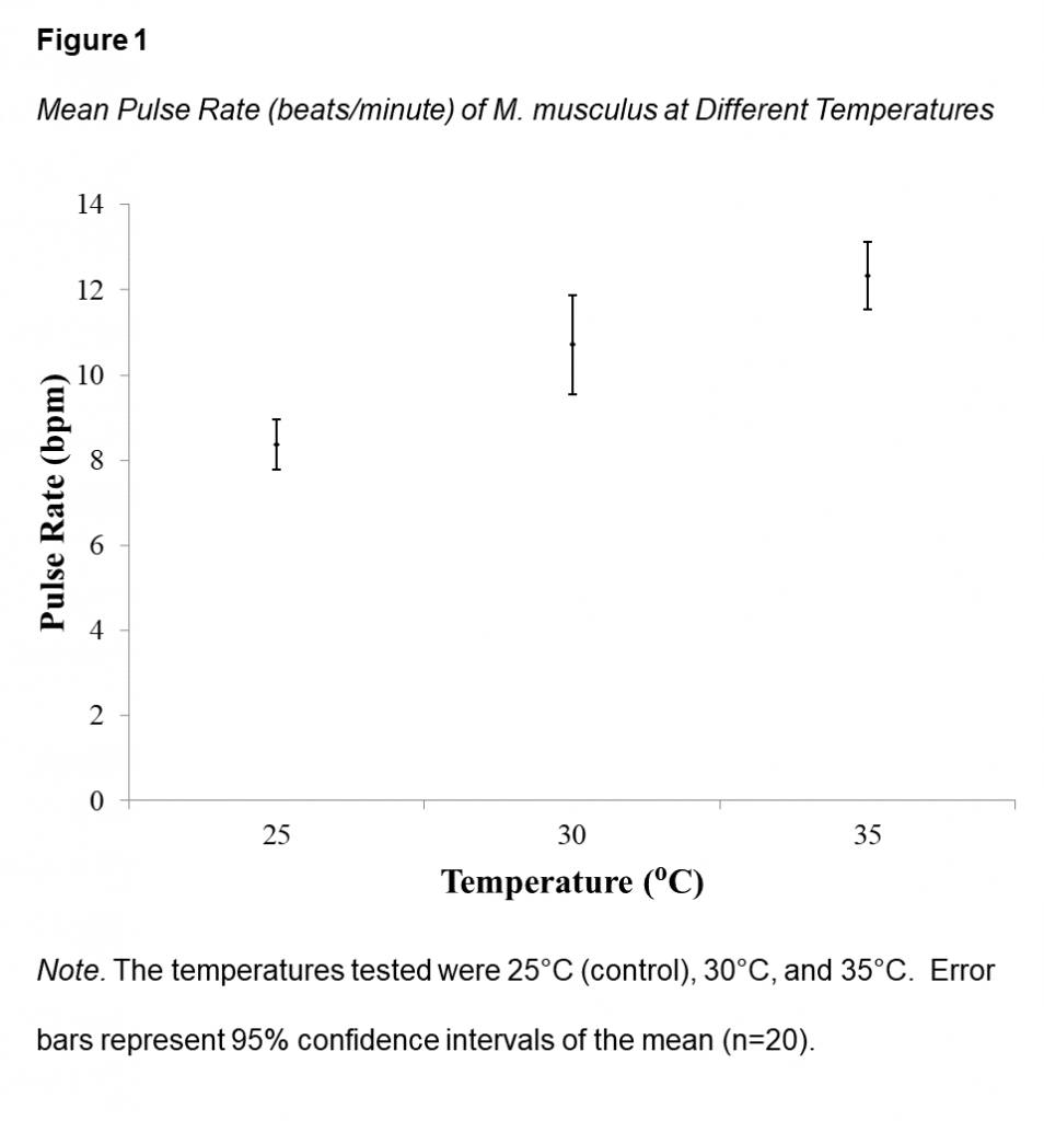
Null hypothesis (H 0 ) : Temperature ( o C) will have no effect on the pulse rate, measured in beats per minute, of mice ( Mus musculus ).

Alternate hypothesis (H A ) : Temperature ( o C) will have an effect on the pulse rate, measured in beats per minute, of mice ( Mus musculus ).

Reject or Fail to Reject the Null Hypothesis

To determine if two groups are different from one another, we look to see whether or not their respective 95% confidence intervals overlap and then relate this conclusion back to our two hypotheses.

If the 95% confidence intervals of two sample means do overlap (e.g., a treatment and the control), we are less than 95% sure (i.e. not sure enough) that these two groups reflect a true difference in the populations. This results in a failure to reject the null hypothesis , as there is insufficient evidence to support our alternative hypothesis that there was an effect.

If the 95% confidence intervals do not overlap, we are 95% sure that these two groups reflect a true difference in the populations. This result allows us to reject our null hypothesis and provide support for our alternative hypothesis. It should be noted that calculating confidence intervals only allows us to compare two groups at one time.

Interpreting Confidence Intervals

For example, the 95% confidence intervals of the 30 o C and 35 o C degrees treatment groups do not overlap with the confidence intervals of the 25 o C (control) (Figure 1). In this case, we reject the null hypothesis and provide support for the alternate hypothesis. We conclude that temperature ( o C) will have an effect on the pulse rate, measured in beats per minute, of mice ( Mus musculus ).

how to write null and alternative hypothesis in latex

How to Address the Null and Alternate Hypotheses in the Discussion

In the Discussion section of your report you will need to discuss whether or not the 95% confidence intervals of the treatment groups overlap with the control.

When addressing the null and alternate hypothesis in the Discussion:

State whether the confidence intervals overlap with the control (be specific about which treatment(s) overlap).
If you reject or fail to reject the null hypothesis (use this language).
A full restatement of the supported hypothesis.

Click on the hotspots below to learn about how to address the null and alternate hypotheses in the Discussion.

How to Address the Null & Alternate Hypotheses in the Discussion

Share This Book

Thank you for visiting nature.com. You are using a browser version with limited support for CSS. To obtain the best experience, we recommend you use a more up to date browser (or turn off compatibility mode in Internet Explorer). In the meantime, to ensure continued support, we are displaying the site without styles and JavaScript.

View all journals
Explore content
About the journal
Publish with us
Sign up for alerts
Open access
Published: 20 August 2024

Flowable composite as an alternative to adhesive resin cement in bonding hybrid CAD/CAM materials: in-vitro study of micro-shear bond strength

Eman Ezzat Youssef Hassanien ORCID: orcid.org/0000-0001-5936-6478 1 &
Zeinab Omar Tolba ORCID: orcid.org/0000-0002-6573-8394 2

BDJ Open volume 10 , Article number: 66 ( 2024 ) Cite this article

Metrics details

Bonded restorations
Fixed prosthodontics

To assess the micro-shear bond strength of light-cured adhesive resin cement compared to flowable composite to hybrid CAD/CAM ceramics.

Materials and methods

Rectangular discs were obtained from polymer-infiltrated (Vita Enamic; VE) and nano-hybrid resin-matrix (Voco Grandio; GR) ceramic blocks and randomly divided according to the luting agent; light-cured resin cement (Calibra Veneer; C) and flowable composite (Neo Spectra ST flow; F), resulting in four subgroups; VE-C, VE-F, GR-C and GR-F. Substrates received micro-cylinders of the tested luting agents ( n = 16). After water storage, specimens were tested for micro-shear bond strength (µSBS) using a universal testing machine at 0.5 mm/min cross-head speed until failure and failure modes were determined. After testing for normality, quantitative data were expressed as mean and standard deviation, whereas, qualitative data were expressed as percentages. Quantitative data were statistically analysed using Student t test at a level of significance ( P ≤ 0.05).

Group GR-F showed the highest µSBS, followed by VE-C, VE-F and GR-C respectively, although statistically insignificant. All groups showed mixed and adhesive failure modes, where VE-F and GR-C showed the highest mixed failures followed by GR-C and VE-C respectively.

Conclusions

After short-term aging, flowable composite and light-cured resin cement showed high comparable bond strength when cementing VE and GR.

An in vitro assessment of the physical properties of manually- mixed and encapsulated glass-ionomer cements

Comparative evaluation of shear bond strength of calcium silicate-based liners to resin-modified glass ionomer cement in resin composite restorations - a systematic review and meta-analysis

In vitro shear bond strength over zirconia and titanium alloy and degree of conversion of extraoral compared to intraoral self-adhesive resin cements

Introduction.

Conservative restorations; such as laminate veneers and occlusal veneers, became highly desired nowadays. Such restorations provided maximum tooth preservation and high patients’ satisfaction [ 1 ]. Wide variety of new CAD/CAM materials has been developed to be used in fabricating such restorations aiming to attain high aesthetics while maintaining optimum mechanical properties.

Conventional ceramics offer excellent aesthetics, colour stability, biocompatibility and serviceability [ 2 , 3 ]. However, their brittleness and the possibility of wearing the opposing dentition during mastication made their use challenging [ 2 , 3 ]. On the other hand, composite resin blocks offered good machinability and low wear to the opposing dentition, however, they suffered from increased material wear with loss of surface polish and colour instability [ 2 , 3 ].

Recently, hybrid or resin-matrix ceramics were introduced to combine the advantages of both ceramics and polymers, aiming to imitate the mechanical behaviour of the natural teeth, while maintaining high aesthetics [ 2 ]. Vita Enamic (VE); a polymer-infiltrated ceramic-network material, possessed a unique structure of two three-dimensional interpenetrating networks comprising a dominant ceramic network (86 wt%) and a polymer network (14 wt%) [ 4 , 5 ]. Voco Grandio (GR), a nano-hybrid resin-matrix ceramic, also consisted of predominant inorganic fillers (86 wt%) in addition to the organic portion [ 6 ].

Both VE and GR offered reduced brittleness [ 2 ], high resilience, flexibility and fatigue resistance [ 6 ] to better withstand the exerted masticatory forces compared to conventional ceramics. They also offered good bond strength and wear resistance with low abrasion to the opposing teeth [ 2 , 6 ]. Being supplied as CAD/CAM blocks, they gained the advantages of the digital workflow, which allowed the production of restorations with high precision and accuracy in short time compared with the conventional approach [ 3 , 7 ]. In addition, compared to conventional ceramic materials, they offered fast machinability without the need of additional firing, glazing or crystalizing procedures [ 2 , 6 ]. Furthermore, they allowed easy intra-oral reparability and polishing [ 6 ], which aided in time-saving and ease of construction.

However, long-term survival of conservative indirect restorations does not depend solely on the restorative material used. It depends greatly on establishing an efficient bond between such restorative material and the prepared tooth structure [ 8 ]. Poor bonding might decrease the restoration fracture strength, retention and increase the risk of micro-leakage [ 6 , 9 ].

For many years, light-cured adhesive resin cement was the material of choice when cementing conservative indirect aesthetic restorations, owing to their high mechanical properties, low solubility, high colour stability and controllable working time [ 10 , 11 , 12 , 13 , 14 ]. However, their use possessed some challenges, where improper handling might cause premature curing with or without the presence of excess cement residing in undesirable areas and difficult to remove. Additionally, their relatively low inorganic filler content, which contributes to their high flow, could increase the volumetric polymerization shrinkage and result in a thermal expansion coefficient higher than that of enamel and dentin, which can subsequently result in interface failure; exposing the cement to the oral environment and compromising the restoration longevity and aesthetics [ 14 , 15 ].

On the other hand, dual-cured resin cements possessed higher mechanical properties; such as flexural strength, hardness and elastic modulus, when compared to light-cured resin cements [ 10 , 13 ]. They also showed a higher degree of conversion [ 10 , 13 ] due to their dual activation modes, with better physicochemical properties [ 10 ]. However, these cements suffered from a shorter working time and colour instability [ 10 , 13 ], which possessed a problem in aesthetic restorations. Hence, alternative materials were investigated.

Some researchers speculated that using composite resins; with higher inorganic filler content [ 10 , 14 , 16 ] and lower initiators concentration [ 14 ], might be advantageous in all ceramic restorations cementation, because they possessed higher colour stability and mechanical wear resistance [ 14 , 16 ] compared to dual-cured resin cements. However, such increase in the filler content increased the material viscosity, which represented a challenge during restoration seating and caused a thick cement line at the interface [ 16 ].

Hence, attempts were made to reduce such viscosity by preheating. It was believed that preheating can improve the material flow [ 16 ]; allowing better restoration adaptation [ 10 ], thin cement line [ 16 ], lower defects at the margins [ 10 ], and increased degree of conversion with better physical and mechanical properties at low cost [ 10 ].

However, preheating is technique sensitive [ 14 ] and added an additional step to the clinical procedure [ 14 ], which is considered a limitation. Additionally, it was found that the preheating effect varied according to the resin composite type [ 10 , 15 , 16 ], composition [ 10 ], filler content and size [ 10 , 16 ], and photo-initiator system [ 10 ]. Some researchers found that preheated nano-hybrid resin formed a thicker film than that formed by preheated micro-hybrid resin [ 16 ]. Preheating temperature and time [ 16 ] is also an affecting factor; where different composite resins take different times to reach a stable temperature. Additionally, prolonged heating in ovens or warmers can cause some low molecular weight components of the photo-initiator system to volatilize [ 16 ]. Although increasing the degree of conversion by preheating can reduce the light-polymerization time, ideal light-polymerizing time or intensity has not yet been determined [ 16 ]. Furthermore, cementation with preheated composite resins requires higher pressure during the restoration placement, thus, in case of very thin veneers, the possibility of crack and fracture increases [ 10 ]. Hence, using materials that possess high filler content with high flow and do not require additional preheating step; such as flowable composites, might be beneficial.

Flowable composites were first introduced as conservative restorative materials, cavity liners, pits and fissure sealants [ 17 ]. However, their use has expanded lately to involve other applications including orthodontic bracket and retainer bonding, splinting fractured teeth, repairing provisional restorations and recently veneers cementation [ 13 , 17 , 18 ]. Flowable composite, is an adhesive material, with particle size similar to that of the hybrid composites but possesses lower viscosity while maintaining excellent handling properties [ 13 , 17 ]. Their remarkable effective penetration of surface irregularities with adequate surface wetting ability [ 13 , 18 , 19 ], radio-opacity, shade variety and improved cost benefit compared to resin cements made them a valuable alternative to adhesive resin cement in luting conservative restorations [ 13 , 18 ]. Both light-cured resin cements and flowable composites contained low concentration of tertiary amines offering greater colour stability compared to dual-cued resin cement [ 8 ].

Compared to resin cements, the advantages of flowable composites lie in combining higher filler content with low viscosity and clinical procedures simplicity at lower cost. The higher filler content is beneficial in improving their physical properties [ 20 ], which might aid in indirect conservative restoration longevity. Their viscosity facilitated pre-polymerization clean-up without the need for partial or tack polymerization employed in resin cements [ 21 ] in addition to allowing low film thickness and facilitating thin restoration seating [ 15 ] with minimum pressure. Furthermore, their high flexibility allowed them to be less prone to displacement in high-stress areas [ 19 ]. It was also believed that their use can prevent bubble incorporation or entrapment [ 21 ], which might occur when using resin cements that employ mixing two components [ 14 ].

Several studies were conducted to test the efficiency of using flowable composite as a luting agent compared to resin cements, regarding different parameters such as colour stability and opacity [ 13 ], micro-tensile bond strength [ 22 ], compressive strength [ 23 ], radiant exitance, degree of conversion [ 15 , 24 ], shrinkage strain, polymerization stress, elastic modulus [ 15 ], florescence [ 20 ] and shear bond strength to feldspathic porcelain [ 21 ] and lithium disilicate [ 18 ]. However, the difference between their bondability to polymer-infiltrated ceramic network and nano-hybrid resin-matrix ceramic is still unclear.

To test bonding in-vitro, several tests were commonly used, including shear, micro-shear, tensile and micro-tensile bond strength tests. Micro-shear bond strength test (μSBS) offered simple testing protocol, with good control on the bonded area by using standardized micro-tubes of known diameter [ 25 , 26 , 27 ].

For better simulation of intra-oral conditions, aging is usually employed in in-vitro studies. Water storage, a popular aging method, offered an easy, simple, low-cost method with a well-known effect on degrading bonded interfaces [ 28 ]. The high molar concentration of water and its small molecular size allowed its penetration in the small spaces between the polymer chains or functional groups, which deteriorated the polymer thermal stability causing its plasticization and subsequently hydrolytic degradation of resin luting agents [ 29 ]. Hence, it was employed in many in-vitro studies that tested bonding strength.

To the best knowledge of the authors, limited data are available comparing flowable composite bonding performance to that of adhesive resin cement especially when using advanced ceramic materials. Thus, the present study aimed to evaluate the micro-shear bond strength of flowable composite to recent CAD/CAM materials (VE and GR) in comparison to adhesive resin cement after aging. The first tested null hypothesis was that there would be no statistically significant effect of the luting material on micro-shear bond strength of VE and GR materials, while the second null hypothesis was that, regardless of the luting material used, there would be no statistically significant difference between the bond strength of either VE or GR.

The study design, ethical approval, and sample size calculation

The present study is an in-vitro research performed in a randomized and blinded manner. The study received ethical approval from the Ethics Committee of Scientific Research—Faculty of Dentistry—Cairo University.

Prior to conducting the study, sample size calculation was performed using PS: Power and Sample Size Calculations software (version 3.2.1, Vanderbilt University), adopting 0.05 alpha level of significance and a power of 80% rendering a total of 64 samples.

The materials used in the present study, their description, composition, manufacturer and batch number are listed in Table 1 ; whereas, the study experimental design is shown in Fig. 1 .

(VE VITA Enamic, GR Voco Grandio).

Substrates preparation

Two groups of rectangular-shaped discs (12 × 14 × 2 mm) were obtained from VITA Enamic (VE; VITA Zahnfabrik, Bad Säckingen, Germany) and Voco Grandio (GR; VOCO GmbH, Cuxhaven, Germany) blocks using linear precision cutting machine (IsoMet 4000, Buehler, USA) at low-speed of 2500 rpm under copious water to avoid heat generation [ 17 , 30 , 31 ].

All discs were inspected for any evident defects and checked using a precise digital caliper (Digital Vernier Caliper IP54, USA) to verify their thickness. Defect-free discs were individually embedded in auto-polymerizing acrylic resin (Acrostone, Acrostone Co Ltd, Egypt) block to facilitate their handling and testing. All substrates were ultrasonically cleaned (CODYSON, CD-4820, China) in distilled water [ 6 ] for 10 min and air-dried [ 30 , 32 ] to eliminate any residual debris. Each substrate was then placed in a small numbered sealed plastic bag to protect its bonded surface from scratching or contamination and to help in randomization and blinding.

Substrates randomization and subgrouping

Each group of substrates was randomly divided into two subgroups according to the luting material tested ( n = 16 per subgroup); VE-C: VE discs receiving light-cured resin cement, VE-F: VE discs receiving flowable composite, GR-C: GR discs receiving light-cured resin cement, and GR-F: GR discs receiving flowable composite. Randomization of substrates was performed using randomized sequence lists generated using computer software ( www.random.org ) to ensure bias elimination and guarantee results reliability.

Substrates surface treatment

For gr substrates.

The discs’ exposed surface was air-abraded (Basic eco Fine sandblasting unit, Renfert GmbH, Germany) using 50 μm Al 2 O 3 particle at 1.5 bar pressure as recommended by the manufacturer. To standardize the distance between the air-abrading machine nozzle and the substrates at 10 mm, a custom-made holding device was constructed (Fig. 2 ). The device comprised housing for the air-abrading device hand-piece and another for the substrate. Each housing comprised tightening screws to allow proper adjustments. After air-abrasion, Gr substrates were cleaned using steam cleaner (LIZHONG, China) and dried with oil-free air to remove remnants of air-abrasion particles. A bonding agent (Ceramic bond, VOCO GmbH, Germany) was then applied to the air-abraded surface by disposable micro-brush for 60 s and left to dry according to the manufacturer’s recommendations.

GR substrates being air-abraded aided by the custom-made holding device.

For VE substrates

The discs’ exposed surface was etched using 9% buffered hydrofluoric acid (Ultradent Porcelain Etch, Ultradent Products Inc, USA) for 60 s then thoroughly rinsed with water for 20 s and dried for 10 s with oil-free air. Silane coupling agent (Ultradent Silane, Ultradent Products Inc, USA) was then applied to the etched surface with disposable micro-brush and let dry for 60 s.

Preparation of luting agent micro-cylinders

Transparent polyvinyl [ 6 ] tubes of 1.44 mm internal diameter, were cut with the help of an endo-ruler and sharp scalpel (blade #15, Wuxi Xinda Medical Device Co Ltd., China) to obtain equal small micro-tubes of 2-mm height [ 33 ]. The cut micro-tubes were checked meticulously and any micro-tube that showed irregular edges or was cut at an angle other than 90° was discarded and replaced.

Each micro-tube was then placed perpendicular to the bonded surface, held in place with a dental tweezer, and carefully filled with the tested luting material; light-cured resin cement (Calibra Veneer Esthetic Resin Cement, Dentsply, Sirona, Germany) and light-cured flowable composite (Neo Spectra ST flow, Dentsply, Sirona, Germany) by a single skilled operator to ensure standardization. Light-curing (3M ESPE Elipar DeepCure-L, 3M ESPE, St Paul, MN, USA) was performed according to the manufacturer’s instructions for 20 s at each side of the tubes for both materials after excess material removal [ 34 , 35 ].

After complete setting, the micro-tubes were carefully removed after being sectioned with a sharp scalpel (blade #15) [ 6 , 34 ] and the luting material micro-cylinders were checked visually for interface integrity free from air bubbles, gaps, defects or excess material [ 31 ].

Aging and micro-shear bond strength (μ-SBS) test

All specimens in both groups were stored in distilled water at room temperature [ 36 , 37 ] for 21 days to simulate short-term intra-oral aging. A universal testing machine (Model 3345; Instron Industrial Products, Norwood, MA, USA) equipped with a load cell of 5 KN was used to test the micro-shear bond strength. The test was performed by a single assessor, who was blinded to the tested materials with the help of the numbers [ 38 ] that was given to the specimens earlier. The acrylic resin base was secured to the machine’s lower fixed compartment and each bonded micro-cylinder was subjected to a shearing load at a crosshead speed of 0.5 mm/min [ 6 , 39 , 40 ] until failure using orthodontic-wire loop method, where a thin loop-shaped stainless steel orthodontic wire (0.014-inch diameter) was wrapped around each micro-cylinder in contact with the ceramic-resin interface [ 17 , 34 ]. The force required for debonding was recorded in Newton (N) [ 6 , 17 , 34 ] by a computer software (Instron® Bluehill Lite Software). Data were then calculated in mega-pascals (MPa) by the equation:

Where; R : μ-shear bond strength (MPa), F : load to failure (N), A : circular interface area (mm 2 ) calculated by the equation A = πr 2 , where π = 3.14 and r: internal radius of micro-cylinder (0.72 mm) [ 29 , 33 ] resulting in ≈1.63 mm 2 area.

Failure mode/pattern analysis

The debonded surfaces were examined for failure mode determination using a stereomicroscope [ 3 , 6 , 14 , 32 , 41 , 42 , 43 , 44 ] (Leica MZ6, Leica Microsystems, Switzerland) at 20× magnification. The failure modes were classified into; adhesive: at the interface, cohesive: within the luting material or the substrate and mixed: involving both adhesive and cohesive failures [ 6 , 17 , 34 , 45 ]. Representative specimens of different failure patterns were further examined using a high-resolution scanning electron microscope [ 41 , 42 , 44 ] (QUANTA FEG250, FEI Company, Netherlands) at 20 kV and 120× magnification. Both the operator of the stereomicroscope and the operator of the SEM were blinded to the tested groups using the number codes as previously mentioned.

Statistical analysis

Data were statistically analysed by an expert statistician, who was also blinded to the tested groups, using statistical software (IBM SPSS Statistics for Windows, Version 25.0., IBM Corp, USA). After checking for normality using Kolmogorov–Smirnov test, quantitative data were found to be parametric and were expressed as mean and standard deviation (SD) then compared using Student t test. On the other hand, qualitative variables were expressed as percentages. The level of significance was set at P value ≤ 0.05 for the present study.

No pretesting failures occurred during the preparation of the specimens or the μ-SBS testing procedures. Mean and standard deviation (MPa) of the μ-SBS values showed statistically insignificant difference among the tested groups as shown in Table 2 . The failure modes revealed both adhesive and mixed failures in all groups (Fig. 3 ). The majority of mixed failures in all groups were predominantly adhesive (>50% of the bonded surface showed adhesive failure). However, adhesive/cohesive failure within the substrate was seen in two specimens in Group VE-F and one specimen in Group GR-F, predominantly cohesive failure within the luting agent was seen in one specimen in Group VE-C, and adhesive/cohesive failure within the substrate and the luting agent was seen in two specimens in Group GR-C (Fig. 4 ).

The failure modes of the tested specimens.

The adhesive ( a , e ) and mixed ( b : adhesive/cohesive failure within the substrate, c , g : predominantly adhesive, d : predominantly cohesive within the luting agent, f : adhesive/cohesive failure within the substrate and the luting agent) failures observed in the present study shown by SEM at 120× magnification. The red arrows correspond to the adhesive failures, the blue arrows correspond to the cohesive failures within the substrates, the yellow arrows correspond to the cohesive failures within the luting agents. [Note: a , b , c , d are specimens of the VE tested groups, while, e , f , g are specimens of the GR tested groups].

The first and second null hypotheses were accepted, where there was statistically insignificant difference among the tested groups.

The use of hybrid ceramics has increased recently to make use of their benefits; such as high resilience, shock-absorbing properties, high milling efficiency with less marginal chipping and good polishability [ 5 , 6 ].

Although resin cements were the gold standard in cementing these materials, flowable composite has been tested as valid alternative. Flowable composite possessed low viscosity with easy pre-polymerization excess material removal [ 21 ]. In addition, it’s light-cuing nature allowed for good control of the working time [ 21 ]. Although resin cements possess high flow, colour stability [ 14 ], availability in wide range of shades with possible application of try in pastes for better reproduction and visualization of the final shade [ 24 ], its low filler content still represents a challenge [ 14 ]. The increasing interest in using flowable composites for adhesive luting is to benefit from their physical properties; being more filler-loaded than resin cements, and their improved cost benefits compared to resin cements [ 20 ].

Upon comparing the shear bond strength of flowable composite and dual-cured resin cement when being used to cement feldspathic porcelain to bovine enamel, Barceleiro et al. [ 21 ], found an insignificant difference between them with the flowable composite showing insignificantly higher values. Also, Mutlu et al. [ 18 ] found that total etch flowable composites showed higher shear bond strength values after thermocycling when compared to total etch dual-cured resin cements, upon being used to cement lithium disilicate glass-ceramics to human dentin.

However, the bonding behaviour of flowable composite when luting hybrid ceramics was scarce. Thus, the present study was conducted aiming to compare the luting efficiency of flowable composite and light-cured resin cement to two advanced hybrid ceramics.

Bonding tests are commonly used in researches to evaluate the performance of adhesive systems and techniques [ 34 ]. The stronger the bond between the tooth and the restoration, the better it will resist the functional stresses [ 34 ]. Although, shear bond strength test is commonly used [ 34 ], micro-shear test was employed in the present study because it was believed to be more accurate since it tested specimens with small surface area allowing better stress distribution [ 34 ]. It was also preferred over micro-tensile bond strength test because specimen preparation in such test possessed some difficulties, required skill and the tensile forces applied are known to cause micro-cracks formation and propagation in the early stage of the test, increasing pre-test failure incidences [ 6 , 31 , 34 ]. However, micro-shear bond strength values can be affected by specimen geometry and loading configurations [ 34 ]; thus, standardization of all micro-cylinders’ length, diameter and testing procedures was employed in the present study.

To perform a successful micro-shear bond strength test with greater sensitivity and more homogeneous data, the bonding area should not exceed 2 mm 2 [ 44 , 46 , 47 ], hence, the diameter of the micro-cylinders employed in the present study was 1.44 mm, with a total bonding area of ≈1.63 mm 2 . The employed micro-cylinders’ diameter lies within the range used in several previous studies, which utilized 1.4 mm [ 44 , 48 ] and 1.5 mm [ 46 , 47 , 49 ] diameters. Additionally, the utilized micro-tubes internal diameter allowed easier application of the luting agent compared to narrow micro-tubes with diameters smaller than 1 mm [ 50 ].

Water storage was also performed as it is considered one of the simplest methods of aging used to simulate intra-oral conditions, with a dramatic effect on bonding [ 28 , 51 , 52 ]. The number of storage days varied greatly among researches testing bonding to ceramics; ranging from 0.16 up to 730 days [ 51 ]. Although some researchers performed their micro-shear bonding tests only after 24 h (1 day) of water storage; such as Yu and Wang [ 53 ], Andermatt and Özcan [ 40 ], Saglam et al. [ 54 ], and Dos Santos et al. [ 37 ], our test was performed after 21 days of water storage to simulate short-term aging. This came in agreement with Samimi et al. [ 51 ], who used two weeks aging period in deionized water prior to testing micro-shear bond strength. They believed that although short-term water storage might be considered a limitation, the small size of the bonding area might allow faster aging effect [ 51 ].

Since aging is well-known to drastically decrease the bond strength values compared to baseline [ 29 ], the present study was more concerned with comparing the bonding effect of the luting agents to two different substrates; testing two main variables, rather than comparing the aging times or protocols.

Stereomicroscope, a non-invasive magnifying instrument that allowed specimens inspection with better details than naked eyes [ 55 ], was used to detect failure modes. Scanning electron microscope was also used to help better visualization of the microstructure topography of the failed specimens at high resolution and considerable field depth [ 56 ].

Our results showed that there was statistically insignificant difference between the μ-SBS of the light-cured resin cement and the flowable composite tested, which might indicate the reliability of flowable composite as an alternative to the resin cement in terms of bonding. However, the difference in µSBS values among the tested groups might be due to the different nature of the substrates and their interaction with the luting materials, which indicated that the effect of luting agent depends on the ceramic material used [ 33 ].

In the current study, VE-C had higher µSBS than GR-C, which came in agreement with Günal-Abduljalil et al. [ 6 ], who found that VE had higher µSBS to dual-cured resin cement after air abrasion and silane application compared to GR. The present results also showed that VE-C had higher µSBS than VE-F, which also agreed with Grangeiro et al. [ 33 ], who found that µSBS of resin cement to VE was significantly higher than flowable composite with or without aging. However, Dikici and Say [ 22 ], found that the flowable composite showed statistically significantly higher micro-tensile bond strength to VE compared to dual-cured resin cement. The difference in their results might be due to using different testing protocol and the different nature of the luting cement.

All µSBS results seen in the present study were higher than the minimum acceptable bond strength values for resin materials to ceramics presented in the literature (10–12 MPa) [ 57 ]. This might be due to employing the surface treatments recommended by the manufacturer for each substrate, which enhanced their bondability. It might also be due to the fact that both the flowable composite and the resin cement had high flow, which enhanced their penetration in the surface irregularities of the pretreated ceramic materials [ 33 ]. This result implicates the reliability of both luting agents in terms of bondability to VE and GR.

The failures seen in the present study were adhesive and mixed in nature, with the majority of the mixed failures being predominantly adhesive. This might be attributed to the low organic content present in both tested substrates; VE and GR, which might have decreased the capacity for chemical copolymerization of free monomers with the luting agent’s monomers [ 43 ].

Our results partially agreed with Beyabanaki et al. [ 43 ], who found that VE showed higher mixed failure than adhesive failures when testing their µSBS to dual-cured resin cement. However, they also found cohesive failures, which was higher than adhesive failure yet lower than mixed failure. The difference in their results might be attributed to the different nature of the luting material; being dual-cured in their study, and the different aging procedures, where they used thermocycling.

However, the present results disagreed with Günal-Abduljalil et al. [ 6 ], who found that both VE and GR had higher adhesive failures than cohesive and mixed failures when testing their µSBS to dual-cured resin cement after air abrasion and silanization, which could be attributed to the difference in the luting agent nature and aging protocol; where they applied water storage for only 24 h.

Although in vitro studies are valuable methods to evaluate dental materials’ behaviour and properties in an easy and rapid manner [ 28 ], they still lack exact simulation of the oral environment conditions. This can be considered a limitation of the present study, which also lacked the simulation of the effect of saliva, cyclic loading and thermal fluctuations. Short-term water storage aging might also be considered a limitation. Hence, further studies are recommended to compare the effect of different storage media, time and temperature on the bond strength of the tested materials, in addition to assessing the colour stability and fracture resistance of variety of ceramic materials cemented using resin cements and flowable composites.

Within the limitations of this in vitro study, it can be concluded that,

Both flowable composite and light-cured resin cement provided high bond strength when cementing VE and GR after short-term aging.

The nature of ceramic material affects its micro-shear bond strength to luting agents.

Data availability

All data included in this study are available from the corresponding author upon request.

Kermanshah H, Borougeni AT, Bitaraf T. Comparison of the microshear bond strength of feldspathic porcelain to enamel with three luting resins. J Prosthodont Res. 2011;55:110–6.

Article PubMed Google Scholar

Conejo J, Ozer F, Mante F, Atria PJ, Blatz MB. Effect of surface treatment and cleaning on the bond strength to polymer-infiltrated ceramic network CAD-CAM material. J Prosthet Dent. 2021;126:698–702.

Article CAS PubMed Google Scholar

Sismanoglu S, Gurcan AT, Yildirim-Bilmez Z, Gumustas B. Mechanical properties and repair bond strength of polymer‐based CAD/CAM restorative materials. Int J Appl Ceram Technol. 2021;18:312–8.

Article CAS Google Scholar

Queiroz-Lima G, Strazzi-Sahyon HB, Maluly-Proni AT, Fagundes TC, Briso ALF, AssunçãoWG, et al. Surface characterization of indirect restorative materials submitted to different etching protocols. J Dent. 2022;127:104348.

Bajraktarova-Valjakova E, Korunoska-Stevkovska V, Kapusevska B, Gigovski N, Bajraktarova-Misevska C, Grozdanov A. Contemporary dental ceramic materials, a review: chemical composition, physical and mechanical properties, indications for use. J Med Sci. 2018;6:1742–55.

Google Scholar

Günal-Abduljalil B, Önöral Ö, Ongun S. Micro-shear bond strengths of resin-matrix ceramics subjected to different surface conditioning strategies with or without coupling agent application. J Adv Prosthodont. 2021;13:180.

Article PubMed PubMed Central Google Scholar

Drumond AC, Paloco EAC, Berger SB, González AHM, Carreira AJ, D’Alpino PHP, et al. Effect of two processing techniques used to manufacture lithium disilicate ceramics on the degree of conversion and microshear bond strength of resin cement. Acta Odontol Latinoam. 2020;33:98–103.

Leal CL, Queiroz APV, Foxton RM, Argolo S, Mathias P, Cavalcanti AN. Water sorption and solubility of luting agents used under ceramic laminates with different degrees of translucency. Oper Dent. 2016;41:E141–E48.

Akah MM, Yousef EE. Effect of air abrasion pressure and CAD/CAM milling on microtensile bond strength of reinforced composite inlays to immediately sealed dentin: an in vitro comparative study. Egypt Dent J. 2022;68:995–1002.

Article Google Scholar

Gugelmin BP, Miguel LCM, Filho FB, Cunha LF, Correr GM, Gonzaga CC. Color stability of ceramic veneers luted with resin cements and pre-heated composites: 12 months follow-up. Braz Dent J. 2020;31:69–77.

Ramos NC, Luz JN, Valera MC, Melo RM, Saavedra GSFA, Bresciani E. Color stability of resin cements exposed to aging. Oper Dent. 2019;44:609–14.

Furuse AY, Glir DH, Rizzante FAP, Prochnow R, Borges AFS, Gonzaga CC. Degree of conversion of a flowable composite light-activated through ceramics of different shades and thicknesses. Braz J Oral Sci. 2015;14:230–3.

Archegas LRP, Freire A, Vieira S, Caldas DBM, Souza EM. Colour stability and opacity of resin cements and flowable composites for ceramic veneer luting after accelerated ageing. J Dent. 2011;39:804–10.

Raposo CC, Nery LMS, Carvalho EM, Ferreira PVC, Ardenghi DM, Bauer J, et al. Effect of preheating on the physicochemical properties and bond strength of composite resins utilized as dental cements: an in vitro study. J Prosthet Dent. 2023;129:229.e1–e7.

Liberato WF, Silikas N, Watts DC, Cavalcante LM, Schneider LFJ. Luting laminate veneers: do resin-composites produce less polymerization stress than resin cements? Dent Mater. 2023;39:1190–201.

Poubel DLDN, Zanon AEG, Almeida JCF, Rezende LVML, Garcia FCP. Composite resin preheating techniques for cementation of indirect restorations. Int J Biomater. 2022;2022:1–10.

Papazekou P, Dionysopoulos D, Papadopoulos C, Mourouzis P, Tolidis K. Evaluation of micro-shear bond strength of a self-adhesive flowable giomer to dentin in different adhesive modes. Int J Adhes Adhes. 2022;118:103188.

Mutlu A, Atay A, Çal E. Bonding effectiveness of contemporary materials in luting glass-ceramic to dentine: an in vitro study. J Adv Oral Res. 2021;12:103–11.

Cheruvathoor JJ, Thomas LR, Thomas LA, Shivanna MM, Machani P, Naik S, et al. Push-out bond strength of resin-modified glass ionomer cement and flowable composite luting systems on glass fiber post of root canal. Materials. 2021;14:6908.

Article CAS PubMed PubMed Central Google Scholar

Pereira JSDC, Reis JA, Martins F, Maurício P, Fuentes MV. The effect of feldspathic thickness on fluorescence of a variety of resin cements and flowable composites. Appl Sci. 2022;12:6535.

Barceleiro MO, Miranda MS, Dias KRHC, Sekito T,Jr. Shear bond strength of porcelain laminate veneer bonded with flowable composite. Oper Dent. 2003;28:423–8.

PubMed Google Scholar

Dikici B, Say EC. Bonding of different resin luting materials to composite, polymer-infiltrated and feldspathic ceramic CAD/CAM blocks. J Adhes Sci Technol. 2021;36:1572–92.

Weng J-H, Chen H-L, Chen G, Cheng C-H, Liu J-F. Compressive strength of lithium disilicate inlay cementation on three different composite resins. J Dent Sci. 2021;16:994–1000.

De Jesus RH, Quirino AS, Salgado V, Cavalcante LM, Palin WM, Schneider LF. Does ceramic translucency affect the degree of conversion of luting agents? Appl Adhes Sci. 2020;8:4.

Fornazari IA, Brum RT, Rached RN, Souza EM. Reliability and correlation between microshear and microtensile bond strength tests of composite repairs. J Mech Behav Biomed Mater. 2020;103:103607.

El Zohairy AA, Saber MH, Abdalla AI, Feilzer AJ. Efficacy of microtensile versus microshear bond testing for evaluation of bond strength of dental adhesive systems to enamel. Dent Mater. 2010;26:848–54.

Cengiz E, Ulusoy N. Microshear bond strength of tri-calcium silicate-based cements to different restorative materials. J Adhes Dent. 2016;18:231–7.

Vilde T, Stewart C, Finer Y. Simulating the intraoral aging of dental bonding agents: a narrative review. Dent J. 2022;10:13.

May MM, Rodrigues CDS, Da Rosa JB, Herrmann JP, May LG. Surface treatment and adhesion approaches on polymer-infiltrated ceramic network: influence on the bond strength to resin cement. Braz J Oral Sci. 2021;20:e211670.

Sarahneh O, Günal-Abduljalil B. The effect of silane and universal adhesives on the micro-shear bond strength of current resin-matrix ceramics. J Adv Prosthodont. 2021;13:292.

Bumrungruan C, Sakoolnamarka R. Microshear bond strength to dentin of self-adhesive flowable composite compared with total-etch and all-in-one adhesives. J Dent Sci. 2016;11:449–56.

Grangeiro MTV, Rossi NR, BarretoLAL, Bottino MA, Tribst JPM. Effect of different surface treatments on the bond strength of the hybrid ceramic characterization layer. J Adhes Dent. 2021;23:429–35.

Grangeiro MTV, Rodrigues CDS, Rossi NR, Souza KB, Melo RM, Bottino MA. Preheated composite as an alternative for bonding feldspathic and hybrid ceramics: a microshear bond strength study. J Adhes Dent. 2023;25:159–66.

Muñoz MA, Baggio R, Mendes YBE, Gomes GM, Luque-Martinez I, Loguercio AD, et al. The effect of the loading method and cross-head speed on resin–dentin microshear bond strength. Int J Adhes Adhes. 2014;50:136–41.

Menon A, Kumar S, Hegde C. Fracture strength of direct and indirect composite veneers after aging: an in vitro study. J Int Oral Health. 2023;15:469.

Monteiro RV, Santos DM, Chrispim B, Bernardon JK, Porto TS, De, et al. Effect of universal adhesives on long-term bond strength to zirconia. J Adhes Dent. 2022;24:385–94.

Dos Santos DM, Monteiro RV, Athayde FRF, De Souza GM. In vitro and practical guide for the analysis of bond strength to ceramics. Ceram Int. 2023;49:17099–108.

Fusco A, Ahmed S, Link J, Al-Talib T, Abubakr NH. Performance of different orthodontic brackets after exposure to dietary components: an in vitro pilot study. Open J Stomatol. 2021;11:341–8.

Saade J, Skienhe H, Ounsi H, Matinlinna JP, Salameh Z. Evaluation of the effect of different surface treatments, aging and enzymatic degradation on zirconia-resin micro-shear bond strength. Clin Cosmet Investig Dent. 2020;12:1–8.

Andermatt L, Özcan M. Micro-shear bond strength of resin composite cement to coronal enamel/dentin, cervical enamel, cementoenamel junction and root cementum with different adhesive systems. J Adhes Sci Technol. 2021;35:2079–93.

Vergano EA, Baldi A, Comba A, Italia E, Ferrero G, Femiano R, et al. Bond strength stability of different dual-curing adhesive cements towards CAD-CAM resin nanoceramic: an in vitro study. Appl Sci. 2021;11:3971.

Celiksoz O, Irmak O. Delayed vs. immediate placement of restorative materials over biodentine and RetroMTA: a micro-shear bond strength study. BMC Oral Health. 2024;24:130.

Beyabanaki E, Eftekhar Ashtiani R, Feyzi M, Zandinejad A. Evaluation of microshear bond strength of four different CAD‐CAM polymer‐infiltrated ceramic materials after thermocycling. J Prosthodont. 2022;31:623–8.

Monteiro RS, Ferrairo BM, Azevedo-Silva LJ, Minim PR, Rubo JH, Furuse AY, et al. Glass ceramics behave like selectively etched enamel on interfaces produced with self-adhesive/ self-curing resin cement. Int J Adhes Adhes. 2023;124:103383.

Liao Y, Lombardo SJ, Yu Q. Argon plasma treatment effects on the micro-shear bond strength of lithium disilicate with dental resin cements. Materials. 2023;16:5376.

Amaral M, Rizzato JMB, Almeida VCS, Liporoni PCS, Zanatta RF. Bonding performance of universal adhesives with concomitant use of silanes to CAD/CAM blocks. Rev Gaúcha Odontol. 2023;71:e20230020.

Münchow EA, Bossardi M, Priebe TC, Valente LL, Zanchi CH, Ogliari FA, et al. Microtensile versus microshear bond strength between dental adhesives and the dentin substrate. Int J Adhes Adhes. 2013;46:95–99.

Mezarina-Kanashiro FN, Bronze-Uhle ES, Rizzante FAP, Lisboa-Filho PN, Borges AFS, Furuse AY. A new technique for incorporation of TiO2 nanotubes on a pre-sintered Y-TZP and its effect on bond strength as compared to conventional air-borne particle abrasion and silicatization TiO 2 nanotubes application on pre-sintered Y-TZP. Dent Mater. 2022;38:e220–e30.

Ayres APA, Hirata R, Fronza BM, Lopes BB, Ambrosano GMB, Giannini M. Effect of argon plasma surface treatment on bond strength of resin composite repair. Oper Dent. 2019;44:E75–E82.

Daher R, Krejci I, Mekki M, Marin C, Di Bella E, Ardu S. Effect of multiple enamel surface treatments on micro-shear bond strength. Polymers. 2021;13:3589.

Samimi P, Hasankhani A, Matinlinna JP, Mirmohammadi H. Effect of adhesive resin type for bonding to zirconia using two surface pretreatments. J Adhes Dent. 2015;17:353–9.

Kumar N, Fareed MA, Zafar MS, Ghani F, Khurshid Z. Influence of various specimen storage strategies on dental resin-based composite properties. Mater Technol. 2021;36:54–62.

Yu P, Wang XY. Effects of surface treatment procedures on bond strength of lithium disilicate glass-ceramic. Chin J Dent Res. 2021;24:119–24.

Sağlam G, Cengiz S, Köroğlu A, Şahin O, Velioğlu N. Comparison of the micro-shear bond strength of resin cements to CAD/CAM glass-ceramics with various surface treatments. Materials. 2023;16:2635.

Patel P, Patel D. Stereomicroscopy—a potential technique for forensic dental profiling. J Microsc Ultrastruct. 2024; 10.4103.

Babarasul DO, Faraj BM, Kareem FA. Scanning electron microscope image analysis of bonding surfaces following removal of composite resin restoration using Er: YAG laser: in vitro study. Scanning. 2021;2021:2396392.

Erdemir U, Sancakli HS, Sancakli E, Eren MM, Ozel S, Yucel T, et al. Shear bond strength of a new self-adhering flowable composite resin for lithium disilicate-reinforced CAD/CAM ceramic material. J Adv Prosthodont. 2014;6:434.

Download references

Open access funding provided by The Science, Technology & Innovation Funding Authority (STDF) in cooperation with The Egyptian Knowledge Bank (EKB).

Author information

Authors and affiliations.

Fixed Prosthodontics Department, Faculty of Dentistry, Cairo University, Cairo, Egypt

Eman Ezzat Youssef Hassanien

Conservative Dentistry Department, Faculty of Dentistry, Cairo University, Cairo, Egypt

Zeinab Omar Tolba

You can also search for this author in PubMed Google Scholar

Contributions

EEYH and ZOT: Conceptualization; Methodology; Validation; Formal analysis; Investigation; Resources; Data Curation; Writing—original draft preparation; Writing—review and editing; Visualization; Supervision.

Corresponding author

Correspondence to Eman Ezzat Youssef Hassanien .

Ethics declarations

Competing interests.

The authors declare that they have no competing interests. The present study is an in-vitro research performed in a randomized and blinded manner. The study received ethical approval from the Ethics Committee of Scientific Research—Faculty of Dentistry—Cairo University.

Additional information

Publisher’s note Springer Nature remains neutral with regard to jurisdictional claims in published maps and institutional affiliations.

Rights and permissions

Open Access This article is licensed under a Creative Commons Attribution 4.0 International License, which permits use, sharing, adaptation, distribution and reproduction in any medium or format, as long as you give appropriate credit to the original author(s) and the source, provide a link to the Creative Commons licence, and indicate if changes were made. The images or other third party material in this article are included in the article’s Creative Commons licence, unless indicated otherwise in a credit line to the material. If material is not included in the article’s Creative Commons licence and your intended use is not permitted by statutory regulation or exceeds the permitted use, you will need to obtain permission directly from the copyright holder. To view a copy of this licence, visit http://creativecommons.org/licenses/by/4.0/ .

Reprints and permissions

About this article

Cite this article.

Hassanien, E.E.Y., Tolba, Z.O. Flowable composite as an alternative to adhesive resin cement in bonding hybrid CAD/CAM materials: in-vitro study of micro-shear bond strength. BDJ Open 10 , 66 (2024). https://doi.org/10.1038/s41405-024-00251-2

Download citation

Received : 13 May 2024

Revised : 12 July 2024

Accepted : 16 July 2024

Published : 20 August 2024

DOI : https://doi.org/10.1038/s41405-024-00251-2

Share this article

Anyone you share the following link with will be able to read this content:

Sorry, a shareable link is not currently available for this article.

Provided by the Springer Nature SharedIt content-sharing initiative

Quick links

Explore articles by subject
Guide to authors
Editorial policies

Stack Exchange Network

Stack Exchange network consists of 183 Q&A communities including Stack Overflow , the largest, most trusted online community for developers to learn, share their knowledge, and build their careers.

Q&A for work

Connect and share knowledge within a single location that is structured and easy to search.

How do I output the hypothesis space symbol?

gives this symbol

while page 3 of https://www.cs.princeton.edu/courses/archive/spring16/cos495/slides/ML_basics_lecture2_linear_classification.pdf

uses this symbol

How do I output the symbol pointed out by the arrow?

Which symbol should I use to denote the hypothesis space?

These slides seem to be made with Powerpoint and its equation editor that has a different font than the standard LaTeX one. – Karlo Commented Jun 24, 2021 at 23:15
2 it's the same thing, just a different font the other characters probably have similar differences – David Carlisle Commented Jun 24, 2021 at 23:23
2 This is a different font’s \mathcal{H} . You can get a list of font specimens from unicode-math and mathalpha . – Davislor Commented Jun 24, 2021 at 23:24

You must log in to answer this question.

Browse other questions tagged symbols ..

The Overflow Blog
Ryan Dahl explains why Deno had to evolve with version 2.0
Featured on Meta
We've made changes to our Terms of Service & Privacy Policy - July 2024
Bringing clarity to status tag usage on meta sites

Hot Network Questions

Negative binomial distributed continuous data for animal modelling
Does the overall mAh of the battery add up when batteries are parallel?
The Master Tetrist
Is it OK to use the same field in the database to store both a percentage rate and a fixed money fee?
Significance of Elijah's and Elisha's Crossing of the Jordan River
Did polls adjust their methodology after overestimating Democrat's shares in the 2016 and 2020 presidential elections in the Rust Belt?
Are ～渋る and ～惜しむ any different as verbal suffixes?
What do all branches of Mathematics have in common to be considered "Mathematics", or parts of the same field?
Do linguists have a noun for referring to pieces of commendatory language, as a sort of antonym of 'pejoratives'?
Is this a real early draft of the script for The Matrix?
block diagonal matrix
Which philosopher, if any, has defined matter as persistence of experience?
Did anyone ever ask Neil Armstrong whether he said "for man" or "for a man?"
How can an Investigator get critical specialization effects on unarmed attacks?
UV Stretching unfounded
Who said "If you don't do politics, politics will do you"?
Fantasy book with king/father who pretends to be insane
Why don't we observe protons deflecting in J.J. Thomson's experiment?
Is this misleading "convenience fee" legal?
dired: How to disable moving the cursor horizontally?
What did Scott Lang mean by "living as a tenant of the state"?
Multiple unds in a sentence
If you get pulled for secondary inspection at immigration, missing flight, will the airline rebook you?
More efficient way to use Symmetrical Difference tool for layer with many features

$how to write null and alternative hypothesis in latex$

IMAGES

Difference between Null and Alternative Hypothesis
Null and Alternative hypothesis
Null and Alternative Hypothesis Examples
how to write null hypothesis with symbols
Research Hypothesis Generator
Hypothesis testing: stating the null and alternative hypotheses

COMMENTS

Hypothesis with amsthm package
Anyway, I've read that I can use the amsthm package to write the hypothesis, but I haven't been able to find a working example. \documentclass[12pt,a4paper,oneside]{book} \usepackage{amsmath,amssymb,amsthm} \newtheorem{hyp}{Hypothesis} \begin{document} \begin{hyp} This is my first hypothesis.
Hypotheses and Subhypotheses with ntheorem
There's no need to keep typing \normhyp and \subhyp. Instead, at the start of a group of sub-hypotheses, you need to type either. if the sub-hypotheses hould share their main counter with the preceding (main) hypothesis. \renewcommand\thesubhyp{\thehyp\alph{subhyp}} The better the answer, the higher the score.
How to write a null hypothesis using the ntheorem package
1. You could set the counter to -1 before the null hypothesis (which will increase it to 0) and then back 1 afterwards: \setcounter{hyp}{-1} \begin{hyp} My null hypothesis. \end{hyp} \setcounter{hyp}[1} That could be inconvenient however if you ever move the placement of the null hypothesis relative to other hypotheses, since you'd then have to ...
Null Hyothesis
Null Hyothesis. Postby sbinsaleem » Wed Aug 07, 2013 11:34 am. Hi, I am trying to write the null hypothesis in the same way, we write the hypothesis using the the \newtheorem{hypothesis}{Hypothesis} micro. The following is an example of hypothesis. Can anybody please let me know how I can renew this command or any micro to have a null ...
9.1 Null and Alternative Hypotheses
Some textbook authors prefer to write the null hypothesis for this example as [latex]H_o:\mu=66[/latex], where 66 is the highest value on the null side. When testing the alternative against the null, if we can reasonably be assured that the unknown parameter is greater than 66, then it's automatically greater than any value less than 66.
8.2 Null and Alternative Hypotheses
The form of the alternative hypothesis depends on the wording of the hypothesis test. An alternative notation for [latex]H_a[/latex] is [latex]H_1[/latex]. Because the null and alternative hypotheses are contradictory, we must examine evidence to decide if we have enough evidence to reject the null hypothesis or not reject the null hypothesis.
Latex for hypothesis testing
paired. H0: there's no difference betwee sample mean and the true mean. H1: the sample mean is lower than the true mean. ˉx = ∑n i = 1xi n. sd = √ ∑ni = 1(xi − ˉx)2 / (n − 1) t = ˉx − 0 sd / √n. Reject H0 if t < tn − 1, α. Fail reject H0 if t > tn − 1, α. CI: ( − ∞, ˉx − tdf, α ∗ sd / √n)
Hypothesis Testing: 2 Means (Independent Samples)
Null and Alternative Hypothesis: In a 2-sample problem, the null hypothesis will always be the assumption that the groups are the same, or that they have the same averages. In this case we are being asked if there is evidence that the distances are different, so the alternative hypothesis uses a [latex]\neq[/latex] symbol.
11.4 One-Way ANOVA and Hypothesis Tests for Three or More Population
Because p-value[latex]=0.0462 \lt 0.05=\alpha[/latex], we reject the null hypothesis in favour of the alternative hypothesis. At the 5% significance level there is enough evidence to suggest that there is a difference in the average GPA of the students in the different programs.
9.1 Null and Alternative Hypotheses
The actual test begins by considering two hypotheses.They are called the null hypothesis and the alternative hypothesis.These hypotheses contain opposing viewpoints. H 0, the —null hypothesis: a statement of no difference between sample means or proportions or no difference between a sample mean or proportion and a population mean or proportion. In other words, the difference equals 0.
9.1: Null and Alternative Hypotheses
Review. In a hypothesis test, sample data is evaluated in order to arrive at a decision about some type of claim.If certain conditions about the sample are satisfied, then the claim can be evaluated for a population. In a hypothesis test, we: Evaluate the null hypothesis, typically denoted with $H_{0}$.The null is not rejected unless the hypothesis test shows otherwise.
Null & Alternative Hypotheses
The null hypothesis (H 0) answers "No, there's no effect in the population." The alternative hypothesis (H a) answers "Yes, there is an effect in the population." The null and alternative are always claims about the population. That's because the goal of hypothesis testing is to make inferences about a population based on a sample.
Null and Alternative Hypotheses
Always write the alternative hypothesis, typically denoted with Ha or H1, using less than, greater than, or not equals symbols, i.e., (≠, >, or <). If we reject the null hypothesis, then we can assume there is enough evidence to support the alternative hypothesis. Never state that a claim is proven true or false.
Formatting Annotations with LaTeX : Hypothesis
To use LaTeX formatting in Hypothesis, simply begin and end the markup with two dollar-signs ( $$ ). For example: $$\sum_{\mathclap{1\le i\le n}} x_{i}$$. You can also use the editor toolbar: Click the ∑ icon and note the prompt to Insert LaTeX. Enter your LaTeX markup between the double-dollar-signs.
amsmath
I'm new with Latex and trying to get four hypotheses in the following style: Hypothesis 1 (H1): This is my first hypothesis. I'm using the amsmath package and the following code: \newcommand{hyp}{Hypothesis} \begin{hyp} This is my first hypothesis. \end{hyp} which gives an output of: Hypothesis 1: This is my first hypothesis.
Null and Alternative Hypotheses
The null and alternative hypotheses are two competing claims that researchers weigh evidence for and against using a statistical test: Null hypothesis (H0): There's no effect in the population. Alternative hypothesis (HA): There's an effect in the population. The effect is usually the effect of the independent variable on the dependent ...
13.5 Testing the Significance of the Overall Model
Because p-value[latex]=0.0017 \lt 0.05=\alpha[/latex], we reject the null hypothesis in favour of the alternative hypothesis. At the 5% significance level there is enough evidence to suggest that there is a relationship between the dependent variable "job satisfaction" and the set of independent variables "hours of unpaid work per week ...
How to Write a Null Hypothesis (5 Examples)
H 0 (Null Hypothesis): Population parameter =, ≤, ≥ some value. H A (Alternative Hypothesis): Population parameter <, >, ≠ some value. Note that the null hypothesis always contains the equal sign. We interpret the hypotheses as follows: Null hypothesis: The sample data provides no evidence to support some claim being made by an individual.
6.3: Introduction to Hypothesis Testing
We will begin by writing some hypotheses: The null hypothesis is the statement of no change (the dull hypothesis). In this context, the proportion of coin spins that land tails up is 50% (the same as flipping a penny). In mathematical symbols, $H_0: p=0.5$ Daquan's claim is what we call the alternative hypothesis. The proportion of coin spins ...
Addressing the Null & Alternate Hypotheses
When addressing the null and alternate hypothesis in the Discussion: State whether the confidence intervals overlap with the control (be specific about which treatment (s) overlap). If you reject or fail to reject the null hypothesis (use this language). A full restatement of the supported hypothesis. Click on the hotspots below to learn about ...
6.4: Hypothesis Tests for a Single Population Proportion
The alternative hypothesis is a claim implied by the research question and is an inequality. The alternative hypothesis states that population proportion is greater than (>), less than (<), or not equal (≠) to the assumed value in the null hypothesis. When a test involves a single population proportion, alternative hypothesis will be one of ...
7.1: Null and Alternative Hypotheses
The null hypothesis ( H0. H 0. ) is a statement about the population that either is believed to be true or is used to put forth an argument unless it can be shown to be incorrect beyond a reasonable doubt. The alternative hypothesis ( Ha. H a. ) is a claim about the population that is contradictory to H0. H 0.
Making a list of hypothesis and references to the hypothesis
It seems that hyperref in combination with ntheorem cause unwanted references in the hypothesis list. The list of hypothesis contains a reference to the chapter (chapter 1) and the hypothesis number (hypo 1.1.) following the hypothesis. If a remove the hyperref package the list of hypothesis appears as I want it to be.
Multi-habitat landscapes are more diverse and stable with improved
If the boxplot overlaps the 1:1, then the observed value falls within the null hypothesis; if it is below, the observed value is less than under the null hypothesis and, if above, more than under ...
Hypothesis listing environment for mathematics paper
The number assigned to a hypothesis should be centred vertically with respect to that hypothesis. LaTeX should (preferably) handle linebreaks, since each hypothesis is mostly words. The left-hand margin should be greater than the usual text margin, so that it's inset a little (like with the enumerate environment)
Flowable composite as an alternative to adhesive resin cement in
The first tested null hypothesis was that there would be no statistically significant effect of the luting material on micro-shear bond strength of VE and GR materials, while the second null ...
How do I output the hypothesis space symbol?
Which symbol should I use to denote the hypothesis space? These slides seem to be made with Powerpoint and its equation editor that has a different font than the standard LaTeX one. This is a different font's \mathcal{H}. You can get a list of font specimens from unicode-math and mathalpha.

LaTeX.org on Twitter - follow us

LaTeX forum ⇒ General ⇒ Null Hyothesis

Who is online

9.1 Null and Alternative Hypotheses

Share This Book

Latex for hypothesis testing

Distribution

Normal Distribution

One Group t-test

right tailed

Two Group testing

t-test with equal variance

t-test with unequal variance

Multigroup Camparison

Proportion testing

Independent test

Fisher Exact

9.1 Null and Alternative Hypotheses

Example 9.1

Example 9.2

Example 9.3

Example 9.4

Collaborative Exercise

Have a language expert improve your writing

Null & Alternative Hypotheses | Definitions, Templates & Examples

Table of contents

Here's why students love Scribbr's proofreading services

Examples of null hypotheses

Examples of alternative hypotheses

Prevent plagiarism. Run a free check.

General template sentences

Test-specific template sentences

Cite this Scribbr article

Is this article helpful?

Shaun Turney

Null and Alternative Hypotheses

Chapter Review

Formula Review

Formatting Annotations with LaTeX

Related Articles

Ask a Question

Have a thesis expert improve your writing

Null and Alternative Hypotheses | Definitions & Examples

Table of contents

Examples of null hypotheses

Examples of alternative hypotheses

Test-specific

Cite this Scribbr article

Is this article helpful?

Shaun Turney

13.5 Testing the Significance of the Overall Model

Testing the Overall Model

Steps to Conduct a Hypothesis Test on the Overall Regression Model

Concept Review

7 Addressing the Null & Alternate Hypotheses

Example of Null and Alternate Hypotheses

Interpreting Confidence Intervals

How to Address the Null & Alternate Hypotheses in the Discussion

Share This Book

Flowable composite as an alternative to adhesive resin cement in bonding hybrid CAD/CAM materials: in-vitro study of micro-shear bond strength

Materials and methods

Conclusions

Similar content being viewed by others

An in vitro assessment of the physical properties of manually- mixed and encapsulated glass-ionomer cements

Comparative evaluation of shear bond strength of calcium silicate-based liners to resin-modified glass ionomer cement in resin composite restorations - a systematic review and meta-analysis

In vitro shear bond strength over zirconia and titanium alloy and degree of conversion of extraoral compared to intraoral self-adhesive resin cements

The study design, ethical approval, and sample size calculation

Substrates preparation

Substrates randomization and subgrouping

Substrates surface treatment

For VE substrates

Preparation of luting agent micro-cylinders

Aging and micro-shear bond strength (μ-SBS) test

Failure mode/pattern analysis

Statistical analysis

Data availability

Author information

Contributions

Corresponding author

Ethics declarations